Modeling Preference Change through Brand
Satiation
著者
TERUI Nobuhiko, HASEGAWA Shohei
journal or
publication title
Discussion Papers (Tohoku Management &
Accounting Research Group)
number
112
year
2013-04
TOHOKU MANAGEMENT
&ACCOUNTING RESEARCH GROUP
Discussion Paper No. 112
Modeling Preference Change
through Brand Satiation
Nobuhiko Terui and Shohei Hasegawa
April, 2013
GRADUATE SCHOOL OF ECONOMICS AND MANAGEMENT TOHOKU UNIVERSITY KAWAUCHI, AOBA-KU, SENDAI 980-8576 JAPAN
1
Modeling Preference Change through Brand Satiation
by
Nobuhiko Terui
Graduate School of Economics and Management Tohoku University
Sendai, Japan
and
Shohei Hasegawa
Graduate School of Economics and Management Tohoku University
Sendai, Japan
2
Modeling Preference Change through Brand Satiation
Abstract
In this study, we develop structural models of preference change due to consumer state dependence through satiation by purchase experience. A dynamic factor model with switching structure is proposed to explain consumer preference changes. Two types of dynamic factor models are separately applied to baseline and satiation parameters in a direct utility model that accommodates multiple discreteness data. The first dynamic factor model has a switching structure for consumer preference, and decomposes brand baselines into time-invariant factor loadings for the coordinates of brand positions and time-varying factor scores for consumer preference directions. The second dynamic factor model applied to satiation parameters extracts the consumer level of satiation in a product category, and this is used as a causal variable in a switching equation to show when and how preferences change over time according to the level of brand satiation. The brand positions and temporal changes of heterogeneous preferences are jointly depicted in a dynamic joint space map.
The empirical analysis of a panel dataset shows that our proposed dynamic model, implying that consumers change their preferences when previous brand satiation exceeds the admissible level and preference directions are determined by the previous level of satiation, performs better than alternative specifications, such as a static model with no preference change and a dynamic model without structures which imply that preference changes whenever a consumer purchases a product.
Key words and phrases:
Structural Modeling, Brand Positioning, Consumption Experience, Joint Space Map, Dynamic Factor Model, Multiple Discreteness Data, Satiation, Switching Structure
3
Modeling Preference Change through Brand Satiation
1. Introduction
Satiation through consumer experience has been discussed in several ways by using different definitions and for different purposes. The first stream of research on satiation is related to
consumer brand-switching behavior in a category that has been discussed in the literature and labeled as variety seeking, e.g., Bawa (1990), Jeuland (1978), Lattin (1987), Johnson, Herrmann, and Gutsche (1995), McAlister (1982), and Lattin and McAlister (1985). These studies assume that
variety-seeking behavior is caused by the satiation dynamics of the desired attributes at a given time and that consumers switch brands when the inferential attribute, such as caffeine in the drink category in McAlister (1982), is satiated. They investigated their hypotheses on the basis of experimental data.
The second stream of research on satiation is related to intertemporal choice. Satiation is defined as the factor of carryover effect of consumption from one period to the next. Brand satiation decreases the utility incorporating satiation due to previous consumption, which is called the
discounted utility model in Baucells and Sarin (2007). This is extended to a model that captures the effect of past consumption by the habituation model, e.g., Wathieu (1997, 2004) and Baucells and Sarin (2010). These analyses are conducted on the basis of a normative approach by using analytical models.
The third stream of research on satiation is related to an economic model with diminishing return of marginal utility proposed by Kim et al. (2002, 2009), where the satiation parameter means the curvature of an direct utility function to explain consumer multiple-choice behavior. Satiation therein is related to the effect of broadening the width of choice. In particular, Hasegawa et al. (2012) proposed the model extracting dynamic satiation score for individual consumer by using dynamic factor model in a choice model which accommodates multiple discreteness data with direct
4
utility. They proposed a model in which dynamics allow the factor scores to evolve over time, reflecting variation in household satiation sensitivity. The analysis of a panel dataset of corn chips purchases indicates that respondent satiation is better explained by a low-dimensional factor structure, leading to implications for product line assortment in the face of quickening satiation.
In this study, we investigate change in consumer preference from the point of view of satiation due to purchase experience. We propose a model to decompose baseline parameters of a direct utility function into time-invariant factor loadings representing brand positions, and a time-varying factor score, the weight of the lower-dimensional axis, and therefore, the preference direction in a lower-dimensional attribute space.
This is an extension of the concept and models for analyzing market structure in the literature called a joint space map, and originally proposed by Hauser and Shugan (1983). Several extensions are found in the following studies. Elrod (1988) proposed a perceptual map model based on
consumer-choice behavior by employing factor analytic decomposition of a brand-specific intercept in the utility function. Chintagunta (1994) extended the model to heterogeneous consumers grouped into a finite number of segments. Erdem (1996) incorporated a higher level of heterogeneity in the model to give continuous mixture models, where heterogeneous parameters were integrated by the simulated maximum likelihood method, leading only to homogeneous model parameter estimates. Moreover, the time-varying intercept connecting to last purchase behavior is incorporated such that the intercept value increases if the same brand is chosen as the last purchase and vice versa; and brand-loyal consumers or variety seekers are identified by reviewing this data, although the brand positioning as well as preference vectors are time invariant. Recently, focusing on the effect of new product entry on market structure, Rutz and Sonnier (2011) proposed a choice model to represent the dynamic change of brand positions, where consumer preference is kept constant.
Most previous studies assume that consumer preference is independent of previous behavior, and that choice is driven temporally by marketing strategies such as pricing and promotions. In this
5
study, we relax this assumption in a way that preference is state dependent similar to the case in Erdem (1996), and propose a model to test the hypothesis that preference changes in the process of purchase experience, and explore the structure when it occurs.
Our model extends those in previous studies in several ways. First, our model is an extension to the dynamic model describing market structure in terms of product and consumers. Second, our model accommodates individual consumer heterogeneity, and then we depict the dynamic joint space map for an individual consumer. Third, we incorporate a mechanism to switch the preference direction in a model, i.e., we develop structural modeling of preference change in a testable way empirically by the data.
As a contribution of structured choice modeling, we incorporate two types of dynamic factor models in a choice model with a direct utility function that accommodates multiple discreteness data. Then, the factor score extracted by the dynamic factor model applied to satiation parameters drives the change of preference direction, which is defined by factor score vector from the second dynamic factor model applied to baseline parameters. Preference changes when the satiation level in the previous state exceeds the admissible range, and it does not change otherwise. We compare the model with alternative models, which are categorized by “dynamics” and “structure.” This includes the model without state dependence, i.e., the steady preference model, the dynamic model without structure which implies that preference changes whenever a consumer purchases a product.
The remainder of this article is organized as follows. In section 2, we present the models by defining the utility function and distributional assumptions of the model variables as well as related comparative models. Section 3 describes the empirical results of an application of the proposed model to a panel dataset of corn chips purchases. In section 4, we discuss implications, and section 5 concludes this study with a summary. The algorithm for model estimation and parameter
6
2. Model
Utility Function and Likelihood
We employ the utility function proposed by Bhat (2005) and used in Hasegawa et al. (2012) by incorporating product attributes and dynamic effects in the baseline utility and satiation parameters. Consumer h’s utility over j 1, … , m varieties at time t are defined as follows:
U , z ∑ ln γ x 1 ln z , (1)
where x , … , x is the vector of quantity demanded by consumer h at t, z
represents the outside good, and ψ , γ j 1, … , m are parameters restricted as ψ 0 and γ 0. ψ is the baseline value of marginal utility for a product j when x 0, and γ is a satiation parameter that affects the rate at which marginal utility diminishes.
The stochastic model is obtained by assuming that the baseline utility parameter has an error, or that ψ exp ψ ε where ψ and ε are unrestricted and independent errors,
respectively. Then, the likelihood function is obtained by maximizing (1) subject to the budget
constraint ′ z E , where and , respectively, mean price and quantity vector, and E is the total expenditure. This is accomplished by creating the auxiliary equation as follows:
Q U , z λ ′ z E . (2)
By employing the Kuhn–Tucker conditions of constrained utility maximization, we obtain an expression that relates the observed demand to the error terms as follows:
ε ψ ln γ x 1 ln p
E p′x
if x 0 (3)
ε ψ ln γ x 1 ln
7
Then, the likelihood function is composed of a combination of density and mass, arising from the interior and corner solutions, respectively. We assume that it follows independently normal distribution ε ~N 0, 1 , as developed in Hasegawa et al. (2012).
Baseline and Preference Dynamics with Switching Structure
We assume that the baseline parameters are well projected into a lower-dimensional attributed space, as is done in the choice map:
; N 0, V diag v , … , v . (5)
Each row vector of factor loadings matrix defines the coordinate of brand position and
corresponding factor score vector , indicating consumer h’s preference direction at time t. We assume that the preference direction will change when consumer satiation level exceeds the
admissible level r , but does not change otherwise. Then, the first dynamic factor model is described as follows:
f ; N 0, I if f r
if f r , (6)
where β , β ′ and we set the hierarchical model as β N β , 1 k 1, 2. We set r 0 for identification in the empirical application. This formulation is grounded in consumer behavior theory. That is, the existence of threshold r as a reference point to evaluate current status is based on the adaptation-level theory of Helson (1964), and consumer asymmetric response between regimes is supported by the prospect theory of Kahneman and Tversky (1979).
Satiation Dynamics
We relate m satiation parameters to p brand characteristics p using information provided to us by the product manufacturer in a linear mapping, similar to that found in conjoint analysis. They are used as γ c α , and are organized in a matrix form by
8
where γ exp γ , c is a vector of characteristics for the j product of dimension p, and is the matrix constituted by a row vector. Our previous study, Hasegawa et al. (2012), shows that the brand characteristics data are well connected to satiation and one factor is appropriate for our dataset used in the empirical application. In addition, it was shown that this information is also effective in allowing us to know how these characteristics affect the demand for a product and whether a subset of characteristics is responsible for satiation for a firm’s offerings.
We next decompose the part worth regarding satiation into a time-invariant factor loading matrix and one-dimensional factor f to define the second dynamic factor model as follows:
f ; N 0, Σ diag σ , … , σ (8) f f ν ; ν N 0,1 . (9) Specification (9) defines a non-parametric model for temporal dynamics, and it accommodates a trend component locally over time in the non-stationary part worth and satiation parameters. (See the literatures in time series analysis, e,g, Harvey, A.,1989, Kitagawa and Gersh,1984 and West and Harrison ,1997) The factor score moves more smoothly when the variance of factor score is smaller than the part worth’s variance, as is employed and discussed in Terui et al. (2010) and Hasegawa et al. (2012).
Alternative Models
We compare our model with six alternative models. The first model is static on the preference direction defined by the ordinary factor model, and is denoted as (Static).
; N 0, V diag v , … , v . (10)
The second alternative is the dynamic model as follows:
; N 0, I . (11)
This is non-parametric modeling of a stochastic trend in time series , and is called smoothness prior in state space modeling. We call this model as “non-structured” in the sense that there are no
9
causal variables or structural parameters in the equation. We call the model represented by equation (11) a non-parametric dynamic factor model (NDF). This specification was successfully employed in Hasegawa et al. (2012) to capture the locally linear stochastic trend for a non-stationary series.
The third model describes that the preference direction has a structural equation that is determined by satiation at a previous period as a causal variable:
h1fht 1 ; N 0, I . (12) We call the model represented by (12) as the structured dynamic factor model (SDF). Both the NDF and SDF have a common property that preference changes whenever a consumer purchases a product. The next class of models has a switching mechanism regarding the timing of preference change. We assume that satiation drives the change when the satiation level exceeds the admissible range, and it does not drive the change otherwise. This class has some variations in types. The first model is an SDF model with switching structure, called a switching non-parametric dynamic model (SSDF1):
; N 0, I if f r
if f r (13)
The second model is our proposed dynamic factor model (SSDF2) shown in (6). The third model is composed of these models, called a hybrid dynamic factor model (SSDF3):
h1fht 1 ; N 0, I if f r
if f r (14)
The fourth model is an autoregressive model (SSDF4):
h1fht 1 h2 ; N 0, I if f r
if f r (15)
These models provide a comprehensive set for assessing the benefit of the proposed dynamic model for describing preference change.
10
3. Empirical Application
Data and Variables Chips Data
Data were obtained through an experiment involving undergraduate students at a large university. Students were included in the experiment if they frequently purchased salty snacks for personal consumption. Students were allocated a $2.00 weekly budget and asked to purchase among eight varieties of corn chips. The offerings were priced at $0.33, allowing the students to select up to six packets each week. The regular price of a corn chips packet was $0.99. The students were told that any unused budget allocation would be paid in cash at the end of the experiment. By offering the chips at reduced prices, we hoped to induce higher levels of consumption, which might provide useful information about satiation. Students were instructed to purchase the chips for their own consumption, not for the consumption of others. These data were previously analyzed by Kim et al. (2009) using a subset of product characteristics and a stationary demand model.
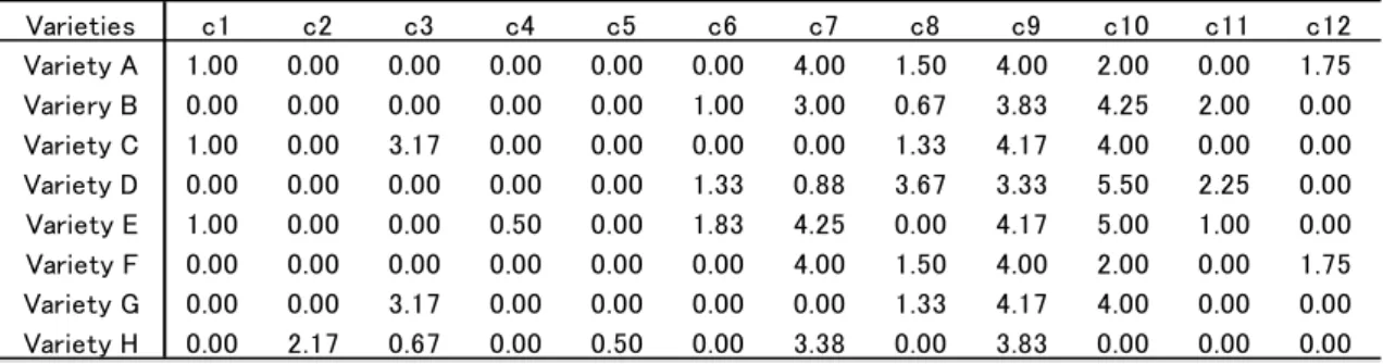
Table 1 lists the offerings and associated product characteristics that were provided by the corn
chips manufacturer. The chip varieties and characteristics are disguised for proprietary purposes, but reflect summary taste characteristics such as “citrus,” “red pepper,” and “treated corn” that are
meaningful to the manufacturer. The experiment was conducted over a seven-week period, resulting in a total of 634 observations for 101 subjects. The data for each purchase occasion is composed of a vector of purchase quantities of each of the eight corn chip varieties, and the quantity of the outside good that was set equal to the unspent budget allocation. Previous analysis of a portion of the characteristics reported in Table 1 indicated that product characteristics could successfully be related to baseline utility in a static model of a choice model.
11
Summary statistics of the data are reported in Table 2. Very few of the purchase occasions resulted in a corner solution where just one of the varieties were selected. Purchase incidence of the varieties ranged from 168 to 244, indicating that no variety was dominant in the data. The
prevalence of interior solutions points to the need for a demand model that can accommodate interior solutions.
== Table 2 ==
Model Comparison
We employ Bayesian MCMC methods to evaluate the joint posterior density for these models. Algorithms for model estimation are provided in the appendix. Models converged relatively quickly and were estimated on the basis of 20,000 iterations of the Markov chain after 10,000 burn-in
samples.The interpretation of satiation parameters and the number of factors are robust throughout the models.
Table 3 reports two measures of model plausibility for each model: the log marginal density (ML) and Bayesian deviance information criterion (DIC). The DIC is a measure of model
comparison that explicitly penalizes a model for its number of parameters (Spiegelhalter et al., 2002). We use the DIC instead of calculating model performance on a holdout set of data because our student panel experienced a fair amount of attrition toward the end of the study, particularly in the sixth and seventh weeks. The loss of data toward the end of the panel makes it difficult to compare the out-of-sample predictions, particularly with dynamic models. The results indicate that the models differ greatly in their fit to the data.
12
First, we find that incorporating dynamics into the baseline parameters ψ leads to a dramatic improvement in model fit in terms of criteria by observing dramatic improvement between the static and dynamic models. The static model fit shows DIC = 11067.6, and log ML = −5088.8. On the other hand, the dynamic models have approximately 80% lesser DIC and 60% greater log ML values.
Second, the comparison among the dynamic models shows that the switching models dominate the steady changing models in both criteria. This means that preference changes occasionally and occurs relative to the level of satiation, which is constituted in the previous period through purchase experience. In addition to the fact that NDF performs slightly better than the causal model (SDF) in steadily changing models, the switching structure with the level of satiation is intrinsic to capture consumer behavior.
Finally, the best model is our proposed model (SSDF2). This means, in addition to the switching mechanism above, that preference change is caused by the previous level of satiation. The next best model is the structured dynamic factor autoregressive model (SSDF4). This means that the
parametric structure works better than non-parametric local trend models (SSDF1 and SSDF3).
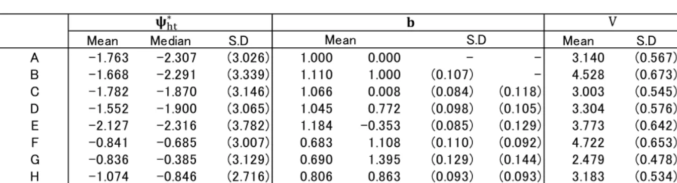
Parameter Estimates
Table 4 summarizes the posterior distributions of parameters for the model SSDF2, the best-fitting model.
== Table 4 ==
First, the bottom portion, Table 4(c), reports estimates of parameters in the second dynamic factor model, i.e., product attribute part-worth on satiation, factor loadings, and variances. The
13
estimates for and have opposite signs, implying that f represents an excitement
(anti-satiation) factor score, the same as that shown in Hasegawa et al. (2012). The estimates of part worth mean the importance weights of product characteristics c1-c12 on the satiation. The
characteristics (c4, c5, c10, c12) have positive large numbers of estimates, implying that these characteristics contribute to brand satiation. In contract, (c1, c8, c11) with negative large values are characteristics which make consumers excitement (anti-satiation). Finally, (c2, c3, c6, c7, c9) have almost zero impact on satiation.
Next, the top portion, Table 4(a), reports estimates of parameters in the first dynamic factor model with switching structure, and the means across households and over time. Since the posterior distributions of some of these quantities are skewed, we also report the posterior median when needed. We observe that the estimated baseline for products are almost proportional to their shares in purchase records. The factor loading matrix , as well as the variance matrix V, are almost significantly estimated. Finally, the middle portion, Table 4(b), reports the posterior mean and median for coefficient parameters in the switching equation. The satiation level f explains the direction of preference in the first dimension as E β 1.323 standard deviation S. D.
0.885 . On the other hand, it does not affect the second dimension as E β 0.112(S.D.:0.854).
== Figure 1 ==
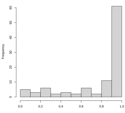
Figure 1 depicts a histogram of individual consumer propensity score k to change their preference. The score is defined by
k T k T (20) where k ∑R k ⁄ is the posterior probability of consumer h’s changing preference at period R t across R iterations of MCMC, and k is the indicator taking binary according to the switching mechanism
14 k 1 if f 0
0 if f 0 (21) The figure shows that many consumers change their preference, as E k = 0.791 and the share of consumers with k 0.8 is 71.3%. On the other hand, it is true that some consumer preferences do not change much.
== Figure 2 ==
Figure 2 shows histograms of estimated coefficients on the switching equation. The left and right figures are the estimates of β for the first dimension of the preference direction and those of β for the second dimension, respectively. The heterogeneous distribution across consumers is relatively stable, although slightly skewed to the right for β . E β 1.323 and E β 0.112. Considering the relation gg ββ f ωω , this means that the satiation level affects the first dimension more than the second dimension.
4. Discussion
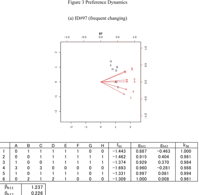
In this section, we investigate the dynamics of preference change by considering three panelists with three patterns that exhibit frequent change of preference over time (panelist #97), moderately frequent change (panelist #35), and not changing (panelist #15), and then consider how estimates for individual consumers are related to observed purchase behavior and switching structure. The dynamic joint space maps are depicted.
Figure 3(a) shows that the preference direction moves every time for panelist #97. The purchase record indicates multiple purchases with a broad range, a satiation score (minus f value) that remains at a high level, and then the switching mechanism works such that the coordinates in the attributed space move all the time. This consumer can be characterized as a variety seeker. The satiation
15
(excitement) level affects both coordinates positively, and this impact is much greater for the first dimension.
== Figure 3 ==
Figure 3(b) provides the map and tables for panelist #35, showing moderately frequent change. Preference changes up to the third time purchase, but does not change anymore after this period. We note that the preference direction is not heading to any product during the first period, and four varieties of corn chips of a single quantity were purchased at this time. This could imply that she was unfamiliar with this product category and getting excited as she purchased them. The satiation (excitement) level negatively and positively affects the first and the second coordinates to change, respectively.
Figure 3(c) provides the map and tables for panelist #15, showing no preference changes. The record for purchasing D is consistent with the preference direction.
The satiation (excitement) level negatively and positively affects the first and second coordinates to change, respectively, and it is much greater for the first coordinate.
5. Concluding Remarks
In this study, we propose a dynamic model of consumer preference change through purchase experience in a direct utility model that accommodates multiple discrete choices. We develop structural modeling of preference in two ways. The first is a cause–effect model of preference directions based on the satiation level in a product category, and the second is a switching structure indicating when the change occurs relative to the level of satiation.
From a modeling perspective, two dynamic factor models are applied to baseline and satiation parameters to extract dynamic factor scores. The first dynamic factor model has a switching
16
structure based on the factor score according to the level of factor score derived from a second dynamic factor model, where the switching occurs when the second score exceeds some admissible level, and it does not occur otherwise. This is motivated by the adaption level theory and the prospect theory for our switching structure. We could furthermore attribute it to the assumption that a consumer has latitude of acceptance for satiation, as satiation and variety-seeking behavior in general, which has been studied extensively in marketing, e.g., McAlister and Pessemier (1982), with taxonomies proposed for explaining variation in consumer choice.
We extensively compare the models, including a static model implying that preference does not change at all, a dynamic model without a switching structure on preference change, and dynamic models with switching structures. The models in the last category are composed of non-parametric local linear trend, parametric regression, and their hybrid models. The measures of model fit, log of marginal likelihood and DIC, support the model with a switching structure and parametric regression. This means that preference will change occasionally after a consumer is satiated enough, and that it stays the same until the critical level.
The empirical application shows that the mode of switching is heterogeneous over consumers. 70 % or more of consumers change their preference by 80% of their purchase opportunities. On the other hand, another portion of consumers is almost uniformly distributed over other levels of change. The investigations of individual consumers are consistent with their choice behavior. That is, the consumer with frequent change of preference has a variety-seeking purchase record with broader range of choices, the consumer not changing preference has a narrow range of choices, and the consumer with moderate preference change behaves in between. Furthermore, the regression coefficients provide useful information on satiation to the coordinates of preference dimensions.
We have some limitations in this research. The empirical findings above are only obtained by applying the model to the dataset we used. The investigation regarding empirical generalization needs more datasets to be analyzed in a variety of categories. When this is done, the causal variable
17
on the structural equation to determine preference as well as switching structure could be different depending on the characteristics of the category. Another limitation is on the modeling. That is, contrary to our assumption of continuous quantity of purchase for analytical equilibrium solutions, we observe a discrete number of purchase quantities. We leave these problems for future research.
18
Appendix – Identification Condition and MCMC Algorithm
We explain the identification condition for the dynamic factor model, and summarize the prior and conditional posterior distribution used for our proposed one-factor model below.
1. Identification Condition on and Priors for Factor Models
For a two-factor model applied to baseline parameters, we restrict the loadings to achieve statistical identification: 1 a 01 a a a a (A.1)
This restriction due to the factor model being applied to parameters of a latent utility is stronger than Geweke and Zhou’s (1996) condition for the conventional factor model.
We then define prior distribution of factor model as:
σ IG n /2, s /2 (A.2) a N a , A ; a , a ′ N , for 3 k p, (A.3) as suggested in Lee (2007).
The first column of (A.1) is set on factor loadings for a one-factor model applied to satiation parameter. The following same prior distributions are employed
v IG n /2, s /2 (A.4) b N b , B for 2 k p, (A.5)
2. Prior Distributions on Hyper Parameters
Prior Setting
a N a , A a 0, A 100
N , , 100
β N β , ν β 0, νβ0 10
19 3. Conditional Posterior Distributions for MCMC
We run 20,000 MCMC iterations for all models, and we used last 10,000 iterations to calculate posterior distribution of model parameters.
(1) | , , , ,
p | , , , ,
det| | ⁄ exp ′ ⁄2
L
(A.6)
The term L is the likelihood function for consumer h 1, … , H at purchase time t 1, … , T , where the likelihood function is composed of a combination of density and mass, arising from the interior and corner solutions, respectively, and is defined as
, … , | | , … ,
See the details in Hasegawa et al. (2012).
Setting r 1, … , R to MCMC iterations, we use Metropolis–Hastings with a random walk algorithm, each h 1, … , H and t 1, … , T .
ψ; ψ N 0, 0.5 (A.7)
The acceptance probability is
min p , , , , p , , , , (A.8) (2) | , , , f , p | , , , f , det| | ⁄ exp f ′ f ⁄2 L (A.9)
As for , we use Metropolis–Hastings with a random walk algorithm, each h 1, … , H and t 1, … , T .
α; α N 0, 0.01 (A.10)
The acceptance probability is
min p , , , ,
20 (3) | , f ,
Under the assumption of uncorrelated a ’s, we define f , f , , f T ′: T 1 matrix, and then make downward stacking over h, ′, ′, ;
H′ ′ : ∏H T 1 matrix. Similarly, we define α , α , … , α T ′: T 1, and ′ , ′ , , H ′ ′ : ∏H T 1. Then, we have the regression equation with coefficient parameter vector and explanatory matrix .
a N a , A , (A.12)
where
A A σ ′ , a A A a σ ′
The identification condition is considered when k 1 .
(4) | , ,
In the same way as , we define , , , T ′: T 2 matrix,
′, ′, ; H ′ ′ : ∏H T 2 matrix and ψ , ψ , … , ψ T ′: T 1, ′, ′, , H′ ′ : ∏H T 1. N , , (A.13) where v ′ , a v ′
The identification condition is considered when j 2 .
(5) f , | , , ,
We reformulate measurement equation (Equations (8) and (13)) and system equation (Equations (9) and (14)). Measurement equation: 0 0 f ; N 0, 0 0 (A.14) System equation: f 1 0 K 1 K f ν ; ν N 0, 10 K0 , (A.15) where β , β ′ and
21
K 1, if f r K 0, if f r ,
(A.16)
where we define f f by interpreting the factor of anti-satiation for f .
We use Carter and Kohn (1994) for a time-varying coefficient in state space model expressed as Equation (A.14) and Equation (A.15)
(6) β , β ′|f , ,
β N β , ′ 1 k 1,2 (A.17)
where
β ′ 1 ′ β
and .
and are the row vector collected in case of regime f r or K 1 . If (K 0 at all t), posterior is β N β , 1 by the homogeneity.
(7) β , β ′|
β N β , H νβ k 1,2 (A.18)
where
22
References
[1] Bawa, K. (1990), “Modeling Inertia and Variety Seeking Tendencies in Brand Choice Behavior,”
Marketing Science, 3, 263-278.
[2] Baucells, M. and R. K. Sarin (2007), “Satiation in Discounted Utility,” Operations Research, 55 (1), 170-181.
[3] Baucells, M. and R. K. Sarin (2010), “Predicting Utility Under Satiation and Habit Formation,”
Management Science, 56 (2), 286-301.
[4] Bhat, C. R. (2005) “A Multiple Discrete-Continuous Extreme Value Model: Formulation and Application to Discretionary Time-Use Decisions,” Transportation Research, 39 (8) 679-707. [5] Carter, C. K. and Kohn, R. C. (1994) “On Gibbs sampling for state space models,” Biometrika,
81, 541-553.
[6] Chintagunta, P. (1994) “Heterogeneous Logit Model Implications for Brand Positioning,”
Journal of Marketing Research, 32, 304-311.
[7] Elrod, T. (1988) “Choice Map: Inferring a Product Market Map from Panel Data,” Marketing
Science, 7, 21-40.
[8] Erdem (1996) “A Dynamic Analysis of Market Structure Based on Panel Data”, Marketing
Science, 15, 359-378.
[9] Geweke, J. and G. Zhou (1996) “Measuring the Pricing Error of the Arbitrage Pricing Theory,”
The Review of Financial Studies, 9, 557-587.
[10] Hasegawa, S., N. Terui and G. Allenby (2012), “Dynamic Brand Satiation,” Journal of
Marketing Research, vol. XLIX, 842-853.
[11] Hauser, J. R. and S. M. Shugan (1983), “Defensive Marketing Strategies,” Marketing Science, 2 (4), 319-360.
[12] Harvey, A. (1989), Forecasting Structural Time Series Models and the Kalman Filter, Cambridge University Press, London.
[13] Helson, H. (1964), Adaption-Level Theory, New York: Harper & Row Publishers, Inc.
[14] Jeuland, A. P. (1978), “Brand Preference Over Time: A Partially Deterministic Operationalization of the Notion of Variety Seeking,” in Research Frontier in Marketing: Dialogues and Directions, No.43, AMA 1978 Educator’s Proceedings, ed. Subashi Jain, Chicago.
[15] Johnson, M. D., A. Herrmann and J. Gutsche (1995), “A Within-Attribute Model of Variety-Seeking Behavior,” Marketing Letters, 6 (3), 235-243.
[16] Kahneman, D. and A. Tversky (1979), “Prospect theory: an analysis of decision under risk,”
Econometrica, 47, 263-291.
[17] Kim, J., G. Allenby and P. Rossi (2002), “Modeling Consumer Demand for Variety,” Marketing
Science, 21, 229-250.
[18] Kim, J., G. Allenby and P. Rossi (2009), “Product attribute and models of multiple discreteness,”
Journal of Econometrics, 138, 208-230.
23
trends and seasonalities,” Journal of the American Statistical Association, vol.79, 378–389. [20] Lattin, J. L. (1987), “A model of Balanced Choice Behavior,” Marketing Science, 6, 48-65. [21] Lattin, J. L. and L. McAlister (1985), “Using a Variety-Seeking Model to Identify Substitute and
Complementary Relationship Among Competing Products,” Journal of Marketing Research, 22, 330-339.
[22] Lee, S.Y. (2007), Structural Equation Modeling: A Bayesian Approach, Wiley, New York. [23] McAlister, L. and E. Pessemier (1982), Variety Seeking Behavior: An Interdisciplinary Review,
Journal of Consumer Research, 9, 311-322.
[24] McAlister, L. (1982), “A Dynamic Attribute Satiation Model of Variety-Seeking Behavior,”
Journal of Consumer Research, 9, 141-150.
[25] Rutz, O. and G. Sonnier (2011), “The Evolution of Internal Market Structure,” Marketing
Science, 30 (2) 274-289.
[26] Spiegelhalter, D. J., N. Best, B. P. Carlin, and A. van der Linde (2002). “Bayesian measures of model complexity and fit,” Journal of the Royal Statistical Society, Series B, 64 (4), 583-616. [27] Terui, N., M. Ban and T. Maki (2010), “Finding Market Structure by Sales Count Dynamics—
Multivariate Structural Time Series Models with Hierarchical Structure for Count Data—,”
Annals of the Institute of Statistical Mathematics, 62, 92-107.
[28] Wathieu, L. (1997), “Habits and the anomalities in intertemporal choice,” Management Science, 43 (11), 1552-1563.
[29] Wathieu, L. (2004), “Consumer habituation,” Management Science, 50 (5), 587-596. [30] West, M and J. Harrison (1997), Bayesian Forecasting and Dynamic Models(2nd
ed.), Springer,
24
Table 1 Product Varieties and Characteristics
Table 2 Purchase Summary
Kim et al. (2007)
Table 3 Model Comparison
Varieties c1 c2 c3 c4 c5 c6 c7 c8 c9 c10 c11 c12 Variety A 1.00 0.00 0.00 0.00 0.00 0.00 4.00 1.50 4.00 2.00 0.00 1.75 Variery B 0.00 0.00 0.00 0.00 0.00 1.00 3.00 0.67 3.83 4.25 2.00 0.00 Variety C 1.00 0.00 3.17 0.00 0.00 0.00 0.00 1.33 4.17 4.00 0.00 0.00 Variety D 0.00 0.00 0.00 0.00 0.00 1.33 0.88 3.67 3.33 5.50 2.25 0.00 Variety E 1.00 0.00 0.00 0.50 0.00 1.83 4.25 0.00 4.17 5.00 1.00 0.00 Variety F 0.00 0.00 0.00 0.00 0.00 0.00 4.00 1.50 4.00 2.00 0.00 1.75 Variety G 0.00 0.00 3.17 0.00 0.00 0.00 0.00 1.33 4.17 4.00 0.00 0.00 Variety H 0.00 2.17 0.67 0.00 0.50 0.00 3.38 0.00 3.83 0.00 0.00 0.00 Varieties Purchase incidence Total purchase quantity Corner solution Interior solution Variety A 168 224 - 168 (1.00) Variery B 177 262 4 (.02) 173 (0.98) Variety C 188 231 - 188 (1.00) Variety D 180 235 - 180 (1.00) Variety E 190 295 2 (.01) 188 (0.99) Variety F 244 446 6 (.02) 238 (0.98) Variety G 235 338 - 235 (1.00) Variety H 218 277 - 218 (1.00) Total 1600 2308 12 (0.01) 1588 (0.99) DIC ML Static 11067.6 -5088.8 NDF (No structure) 8649.0 -3124.5 SDF (Strcture) 8756.7 -3171.8 SSDF1 8435.0 -2829.4 SSDF2 8170.0 -2754.1 SSDF3 8425.9 -2829.5 SSDF4 8283.1 -2758.1 Model Dynamic Steady Switching
25
Table 4 Parameter Estimate
(a) Baseline Parameters
These numbers show the grand mean and median of panelist’s estimates over time across panel members. Number of b and V show the posterior mean and the posterior standard deviation in parentheses.
(b) Switching Equation: Baseline Parameters
These numbers show the grand mean of panelist’s estimates across panel members.
(c) Satiation Parameters: Characteristic Level
These numbers show the grand mean and median of panelist’s estimates over time across panel members. Number of and Σ show the posterior mean and the posterior standard deviation in parentheses.
Mean Median S.D Mean S.D
A -1.763 -2.307 (3.026) 1.000 0.000 - - 3.140 (0.567) B -1.668 -2.291 (3.339) 1.110 1.000 (0.107) - 4.528 (0.673) C -1.782 -1.870 (3.146) 1.066 0.008 (0.084) (0.118) 3.003 (0.545) D -1.552 -1.900 (3.065) 1.045 0.772 (0.098) (0.105) 3.304 (0.576) E -2.127 -2.316 (3.782) 1.184 -0.353 (0.085) (0.129) 3.773 (0.642) F -0.841 -0.685 (3.007) 0.683 1.108 (0.110) (0.092) 4.722 (0.653) G -0.836 -0.385 (3.129) 0.690 1.395 (0.129) (0.144) 2.479 (0.478) H -1.074 -0.846 (2.716) 0.806 0.863 (0.093) (0.093) 3.183 (0.534) Mean S.D V
Mean Median S.D Mean S.D
-1.323 -1.428 (0.885) -1.322 (0.186)
0.112 0.162 (0.854) 0.110 (0.189)
β β
Mean Median S.D Mean S.D Mean S.D
c1 -1.230 -1.396 (1.455) 1.000 - 0.187 (0.058) c2 0.007 0.006 (0.033) -0.003 (0.029) 0.105 (0.026) c3 0.081 0.094 (0.096) -0.064 (0.043) 0.063 (0.012) c4 0.547 0.603 (0.658) -0.441 (0.049) 0.461 (0.107) c5 0.421 0.469 (0.498) -0.336 (0.042) 0.322 (0.056) c6 0.052 0.054 (0.076) -0.042 (0.035) 0.136 (0.024) c7 0.012 0.016 (0.035) -0.010 (0.026) 0.040 (0.006) c8 -0.224 -0.246 (0.262) 0.180 (0.033) 0.069 (0.010) c9 -0.033 -0.033 (0.056) 0.029 (0.020) 0.034 (0.004) c10 0.220 0.253 (0.253) -0.174 (0.037) 0.034 (0.004) c11 -0.129 -0.143 (0.151) 0.102 (0.037) 0.094 (0.019) c12 0.283 0.325 (0.332) -0.226 (0.053) 0.120 (0.028) Σ
26
Figure 1 Preference Change
Figure 2 Parameter Estimates in Switching Equation
Frequency 0.0 0.2 0.4 0.6 0.8 1.0 0 1 02 03 04 05 06 0 1 Frequency −3 −2 −1 0 1 0 5 10 15 20 25 30 2 Frequency −2 −1 0 1 2 0 5 10 15 20 25 30
27
Figure 3 Preference Dynamics
(a) ID#97 (frequent changing)
−2 −1 0 1 2 −2 −1 0 1 2 97 A B C D E F G H −1.0 −0.5 0.0 0.5 1.0 −1.0 −0.5 0.0 0.5 1.0 1 23 4 5 6 A B C D E F G H 1 0 1 1 1 1 1 0 0 -1.443 0.887 -0.463 1.000 2 0 0 1 1 1 1 1 1 -1.462 0.915 0.404 0.981 3 1 0 0 1 1 1 1 1 -1.374 0.929 0.370 0.984 4 3 0 3 0 0 0 0 0 -1.693 0.960 -0.281 0.988 5 1 0 1 1 1 1 0 1 -1.331 0.997 0.081 0.994 6 0 2 1 2 1 0 0 0 -1.309 1.000 0.008 0.961 f g g k 1.237 0.226 β β
28
(b) ID#35 (moderate changing)
−2 −1 0 1 2 −2 −1 0 1 2 35 A B C D E F G H −2 −1 0 1 2 −2 −1 0 1 2 1 2 3 A B C D E F G H 1 0 1 1 1 1 0 0 0 -0.485 -0.162 -0.987 1.000 2 0 0 0 2 3 0 1 0 -0.421 0.977 0.212 0.561 3 0 1 0 0 2 0 2 1 -0.068 0.876 0.483 0.506 4 0 2 1 2 0 0 0 1 0.413 0.933 0.359 0.462 5 1 0 2 2 0 0 0 1 1.066 0.992 0.130 0.433 6 0 0 0 2 0 2 0 2 1.583 0.917 0.400 0.297 f g g k -0.462 0.258 β β
29
(c) ID#15 (not changing)
−2 −1 0 1 2 −2 −1 0 1 2 15 A B C D E F G H −2 −1 0 1 2 −2 −1 0 1 2 1 A B C D E F G H 1 0 1 1 1 1 0 2 0 0.865 0.967 0.254 1.000 2 0 1 0 1 1 0 3 0 0.743 0.942 0.335 0.156 3 0 0 0 3 0 0 3 0 0.548 0.840 0.542 0.198 4 0 0 0 3 0 0 3 0 0.810 0.768 0.640 0.204 5 0 2 0 4 0 0 0 0 0.783 0.815 0.579 0.173 6 0 0 0 4 0 0 2 0 0.666 0.723 0.690 0.152 f g g k -1.147 0.278 β β