2003, Vol. 46, No. 4, 395-408
EXTRACTING FEATURE SUBSPACE FOR
KERNEL BASED LINEAR PROGRAMMING SUPPORT VECTOR MACHINES
Yasutoshi Yajima Hiroko Ohi Masao Mori
Tokyo Institute of Technology Hitachi, Ltd. Keio University
(Received January 15, 2002; Revised June 24, 2003)
Abstract We propose linear programming formulations of support vector machines (SVM). Unlike standard SVMs which use quadratic programs, our approach explores a fairly small dimensional subspace of a feature space to construct the nonlinear discriminator. This allows us to obtain the discriminator by solving a smaller sized linear program. We demonstrate that an orthonormal basis of the subspace can be implicitly treated by eigenvectors of the Gram matrix defined by the associated kernel function. When the number of given data points is very large, we construct a subspace by random sampling of data points. Numerical experiments indicate that the subspace generated by less than 2% of the entire training data points achieves reasonable performance for a fairly large instance with 60000 data points.
Keywords: Support vector machine, kernel function, nonlinear discriminator, feature space, data mining, linear programming
1. Introduction
Recently, support vector machines (SVM) have been studied extensively for classification problems in a variety of areas, such as text categorization [11, 14] and image recognition [8, 22, 23]. In classification problems, a number of labeled data points, called a training dataset, x1, x2, . . . , xM, are given as a set of N dimensional vectors. We assume that a
binary class label yi ∈ {+1, −1} is assigned to each point xi. SVM generates a linear
discriminate function f (x) = wTx − b with a normal vector w ∈ RN and a real number b,
which maps a vector x ∈ RN to a class y ∈ {+1, −1} as follows: y =
(
+1 if f (x) > 0,
−1 if f (x) < 0.
Statistical learning theory [26] indicates that a discriminate function which balances accuracy and capacity must be generated in order to reduce generalization error. To this end, SVM employs convex quadratic programs [15, 21]. The convex quadratic program also plays an important role to generate nonlinear discriminate functions. In order to obtain a nonlinear discriminate function, we consider a nonlinear function φ which maps the data point x into a higher, often infinite dimensional feature space F, in which linear discriminate functions are developed. The problem of finding a separating hyperplane with the largest margin reduces to a quadratic program. The Wolfe dual [17] formulation enables us to formulate the quadratic optimization problems only by the dot product h φ(x) , φ(x0) i in
F, which can be computed directly from the original data points, x and x0, by the kernel functions. The crucial point is that the quadratic optimization problems can be formulated
without involving the explicit calculations of the mapped image φ(x) ∈ F. For instance, polynomial kernels
K ( x , x0) =³xTx0´d,
with an integer parameter d, RBF kernels
K ( x , x0) = exp³−kx − x0k2/σ2´,
with a real parameter σ ∈ R, and sigmoid kernels
K ( x , x0) = tanh³κ xTx0 − Θ´,
with real parameters κ, Θ ∈ R, are commonly used kernel functions. Mercer’s Theorem [27] implies that these functions give rise to nonlinear maps φ(·) for which K ( x , x0) =
h φ(x) , φ(x0) i holds. These kernel-based nonlinear discriminate functions have been
suc-cessfully applied to a number of real-world problems [8, 14, 23].
In the present paper, we propose linear programming approaches for generating kernel-based nonlinear discriminate functions. There are several papers which develop variants of SVMs by solving linear programming problems, including Multisurface Method [20] and Robust Linear Programming (RLP) [2]. One benefit of these approaches is that a linear program is easier to solve compared with a quadratic program. In addition, efficient and robust optimization packages are available. Therefore, the linear programming approach has potential of handling real-world massive datasets. To our knowledge, however, little attention has been given to linear programming approaches, particularly with respect to kernel-based nonlinear discriminate functions. Mangasarian and Musicant [19], Mangasarian [18], and Weston and Watkins [28] have considered nonlinear cases by solving very large linear programs. The number of variables and the number of constraints of these linear programs are roughly proportional to those of training data points, and this can cause computational difficulties in handling huge datasets.
In contrast to these methods, we utilize smaller sized linear programs to generate non-linear discriminate functions. Although the original data points are mapped into the higher dimensional feature space F, a fairly small dimensional subspace can be important in dis-crimination. We will demonstrate that an orthonormal basis of the subspace of F can be implicitly treated by eigenvectors of the Gram matrix defined by the associated kernel func-tion, and that discriminate functions in the subspace are successfully constructed by solving linear programming problems. For the case in which the number of given data points is very large, we develop a technique to compute a subspace of F by random sampling of data points. Our numerical experiments indicate that the subspace generated by less than 2% of the training data points achieves reasonable performance for a huge dataset with 60000 training data points.
The present paper is organized as follows. In Section 2, we briefly review a few variants of SVMs by linear programming including RLP, 1-norm and ∞-norm formulations. Section 3 is devoted to the description of a method for extracting implicitly the orthonormal basis of the subspace of the nonlinear feature space F defined by kernels. We also develop linear programming formulations to generate discriminate functions in this subspace. In Section 4, we present our computational experiments, and concluding remarks are presented in Section 5.
2. Preliminaries
2.1. Linear discrimination
Suppose that we have M data points expressed as vectors of N dimensional real space
RN. We assume that these points are represented by an M × N matrix A, where the
j-th row vector Aj of the matrix A corresponds to the j-th data point. Each point Aj is
associated with either the class +1 or class −1, which is denoted by yj ∈ {+1, −1}. Let y = (y1, y2, . . . , yM)T be an M dimensional vector.
SVMs are used to find a linear discriminate function f (x) = wTx − b with a normal
vector w ∈ RN and a real number b ∈ R such that
Ajw − b ≥ 1 if yj = 1,
Ajw − b ≤ −1 if yj = −1. (2.1)
This condition is equivalently written as follows:
Y (Aw − be) ≥ e, (2.2)
where Y ∈ RM ×M is a diagonal matrix, the diagonal element of which is the vector y, and e is a vector of all ones, the dimension of which is given by context.
The set of points satisfying conditions (2.2) are called linearly separable. In general, however, the normal vector w and the real number b satisfying (2.2) may not always exist. Then, introducing a nonnegative error vector ξ = (ξ1, ξ2, . . . , ξM)T ∈ RM, one can relax
conditions (2.2) to
Y (Aw − be) + ξ ≥ e, ξ ≥ 0. (2.3)
Bennet and Mangasarian [2] considered Robust Linear Programming (RLP) for obtaining the function f (x) = wTx − b by minimizing the total amount of errors as follows:
RLP ¯ ¯ ¯ ¯ ¯ Minimize pTξ
Subject to Y (Aw − be) + ξ ≥ e, ξ ≥ 0, (2.4) where p is a positive weight vector representing misclassification cost.
Based on the idea of structural risk minimization in statistical learning theory, Vapnik [26, 27] showed that generalization ability can be improved by controlling the complexity of the discriminate function, which is characterized by the norm of w. Standard SVMs solve the following quadratic program:
¯ ¯ ¯ ¯ ¯ ¯ Minimize 1 2kwk 2 2+ C0eTξ
Subject to Y (Aw − be) + ξ ≥ e, ξ ≥ 0. (2.5) The associated Wolfe dual [17] formulation [9, 27] is
¯ ¯ ¯ ¯ ¯ ¯ ¯ ¯ ¯ Maximize −1 2α TY QY α + eTα Subject to yTα = 0, 0 ≤ α ≤ C0e, (2.6)
where Q is an M ×M symmetric matrix defined as Q = AAT, and C
0 is a positive parameter
controlling the weight between the error term and the norm kwk which is called the capacity
Several variants of the problem (2.5) have been studied [3, 4, 18, 19, 28] by choosing norms other than the 2-norm in (2.5). In the present paper, we use the formulation based on the 1-norm capacity term i.e., the problem for minimizing C kwk1+eTξ over (2.3). This problem
is formulated as the following linear program: ¯ ¯ ¯ ¯ ¯ ¯ ¯ Minimize C eTs + eTξ Subject to −s ≤ w ≤ s, Y (Aw − be) + ξ ≥ e, ξ ≥ 0, (2.7)
where w ∈ RN, b ∈ R, s ∈ RN and ξ ∈ RM are variables, and C is a positive parameter.
Thus, the dual of this problem is ¯ ¯ ¯ ¯ ¯ ¯ ¯ ¯ ¯ Maximize eTα
Subject to −Ce ≤ ATY α ≤ Ce, yTα = 0,
0 ≤ α ≤ e, where α = (α1, α2, . . . , αM)T is a vector of dual variables.
Let us introduce a new vector of variables β = (β1, β2, . . . , βM)T and let βj = yjαj, j =
1, 2, . . . , M . The dual problem can be equivalently written as ¯ ¯ ¯ ¯ ¯ ¯ ¯ ¯ ¯ Maximize yTβ
Subject to −Ce ≤ ATβ ≤ Ce, eTβ = 0,
0 ≤ Y β ≤ e, which leads to the following formulation:
¯ ¯ ¯ ¯ ¯ ¯ ¯ ¯ ¯ Maximize yTβ Subject to kATβk∞≤ C, eTβ = 0, 0 ≤ Y β ≤ e. (2.8)
Generally, one can also consider the problem with the p-norm capacity term. By using the conic duality [1], primal and dual formulations are given as follows:
¯ ¯ ¯ ¯ ¯ Minimize C kwkp+ eTξ
Subject to Y (Aw − be) + ξ ≥ e, ξ ≥ 0, (2.9)
and ¯ ¯ ¯ ¯ ¯ ¯ ¯ ¯ ¯ Maximize yTβ Subject to kATβkq ≤ C, eTβ = 0, 0 ≤ Y β ≤ e, (2.10)
where k · kq is the conjugate norm of k · kp satisfying q−1+ p−1 = 1. Here, it is worth noting
that problem (2.9) with p = ∞, as well as the associated dual problem (2.10) with q = 1, can also be handled as a linear programming problem. It has been demonstrated [3, 4] that a variant of the problem with the 1-norm capacity term works well, and that, in some cases, it generates better discriminators than that with the ∞-norm.
2.2. Nonlinear discrimination by kernels
Let us now briefly review the idea of generating nonlinear discriminators based on the quadratic programming formulation (2.6), which is employed in standard SVMs. We note that the matrix Q in (2.6) is a Gram matrix [12] of the set of data points A1, A2, . . . , AM
with respect to the usual inner product on RN. Keeping this fact in mind, let us introduce
the nonlinear function φ(x) : RN → F which maps an N dimensional data point x into F, and let K(x, x0) denote the kernel function which gives the inner product of φ(x) and φ(x0) in F. Let K be a Gram matrix of the vectors φ(A
1), φ(A2), . . . , φ(AM) with respect
to the inner product on F. Then, replacing Q with K, we can formulate the problem for discriminating the points in F as the following quadratic programming problem:
¯ ¯ ¯ ¯ ¯ ¯ ¯ ¯ ¯ Maximize −1 2α TY KY α + eTα Subject to yTα = 0, 0 ≤ α ≤ C0e. (2.11)
This problem enables us to construct the discriminate function without explicitly knowing the function φ(·). We refer the reader to [9, 10, 26] and the references therein for a more detailed explanation of the associated primal form of (2.11) and kernel-based nonlinear discriminate functions.
In order to be consistent with the dual formulations described in the previous subsection, let us also introduce a vector of variables β = (β1, β2, . . . , βM)T and let βj = yjαj/C0, j =
1, 2, . . . , M . We then write problem (2.11) equivalently as follows: ¯ ¯ ¯ ¯ ¯ ¯ ¯ ¯ ¯ Maximize −C 2 0 2 β TKβ + C 0yTβ Subject to eTβ = 0, 0 ≤ Y β ≤ e. (2.12)
In the following, we introduce a formulation for the kernel-based nonlinear discriminate functions based on the dual form (2.10) with q = 2. That is, let us consider the problem with the square of the 2-norm capacity constraint defined below:
¯ ¯ ¯ ¯ ¯ ¯ ¯ ¯ ¯ Maximize yTβ Subject to kATβk2 2 ≤ C2, eTβ = 0, 0 ≤ Y β ≤ e. (2.13)
Note that the quadratic constraint can be written as
kATβk2
2 = βTQβ ≤ C2. (2.14)
Replacing Q in (2.14) with the Gram matrix K defined by the kernel function K(·, ·), we obtain the following problem:
¯ ¯ ¯ ¯ ¯ ¯ ¯ ¯ ¯ Maximize yTβ Subject to βTKβ ≤ C2, eTβ = 0, 0 ≤ Y β ≤ e. (2.15)
The next lemma ensures that problems (2.15) and (2.12) are equivalent in the following sense:
Lemma 2.1 For a suitable parameter C, problem (2.15) generates any optimal solutions of
Proof
For any positive parameter C0, let β0 be an optimal solution of (2.12). It is easy to
verify that β0 is also an optimal solution of (2.15) with C2 = β0TKβ0. This completes the
proof. 2
3. Linear Programming Formulations for Kernel SVM 3.1. Eigenvalue decomposition of the Gram matrix
We introduce linear programming formulations for obtaining a discriminate function in the feature space, F, characterized by the kernel function K ( · , · ).
Let λ1 ≥ λ2 ≥ · · · ≥ λM0 > 0 be the positive eigenvalues of the matrix K and
d0
1, d02, . . . , d0M0 ∈ RM be the associated eigenvectors, where the norm of each di is 1.
Also, let us define
D = [d1, d2, . . . , dM0] , where di =
q
λid0i, i = 1, 2, . . . , M0.
Then, the matrix K is decomposed as K = DDT, and the quadratic constraint of the
problem (2.15) can be expressed as
βTKβ = °°°DTβ°°°2 2 ≤ C
2. (3.1)
In many practical situations, the number of data points M is very large. This implies that the number of positive eigenvalues, M0, could also be large. Thus, we will introduce
an approximation to this quadratic constraint. To this end, we consider the largest S ¿ M positive eigenvalues λ1 ≥ λ2 ≥ · · · ≥ λS, and the associated column vectors of D. Then, let
us define a submatrix of D as
DS = [d1, d2, . . . , dS] ,
which results in the following approximation of the quadratic part of problem (2.15):
βTKβ ≈ βTD SDTSβ = ° ° °DTSβ ° ° °2 2.
The symmetric matrix DSDST is the closest matrix to K with rank S in the sense of the
Frobenius norm.
Now, returning to the linear programming scheme, and replacing the Euclidean norm constraint (3.1) with an ∞-norm constraint, we obtain the following problem which can be reduced to a linear program:
¯ ¯ ¯ ¯ ¯ ¯ ¯ ¯ ¯ ¯ Maximize yTβ Subject to °°°DTSβ ° ° ° ∞ ≤ C, eTβ = 0, 0 ≤ Y β ≤ e. (3.2)
As we have seen in Section 2.1, the primal form of this problem (3.2) is: ¯ ¯ ¯ ¯ ¯ ¯ ¯ Minimize C kwSk1+ eTξ Subject to Y (DSwS− bSe) + ξ ≥ e, ξ ≥ 0, (3.3)
where wS ∈ RS, bS ∈ R1and ξ ∈ RM are primal variables. Let us denote an optimal solution
of (3.3) as (wS, bS) = (w∗S, b∗S). We then obtained an optimal linear discriminate function as f (xS) = w∗STxS+ b∗S,
where xS is an S dimensional vector of variables.
3.2. Extracting the subspace of F
Problem (3.3) can be considered as an SVM with a 1-norm capacity term, in which each data point is given as a row vector of the matrix DS, instead of the original data points
given in rows of A. The dimension of the variable wS is, in general, different from that
of the original data points, N. In this subsection, we will introduce several propositions which link the feature space F and the matrix DS. Similar discussions can also be found in
Sch¨olkopf et al. [24].
Let djk denote the jk elements of the matrix DS. Associated with the k-th column vector dk = ( d1kd2k · · · dM k)T of DS, let us define vectors Vk, k = 1, 2, . . . , S in F as follows:
Vk =
PM
j=1djkφ(Aj) λk
, k = 1, 2, . . . , S. (3.4)
Note that since φ(Aj) is not described explicitly, each vector Vk can not be expressed.
The following lemma holds:
Lemma 3.2 The set of vectors { V1, V2, . . . , VS} satisfies h Vk, Vk0i =
(
0 if k 6= k0,
1 o.w,
where h · , · i denotes the inner product defined in F.
Proof
For any k, k0 = 1, 2, . . . , S, verifying that h Vk, Vk0i = 1 λkλk0 M X j=1 M X j0=1 djkdj0k0h φ(Aj) , φ(Aj0) i = 1 λkλk0d T kKdk0 is straightforward. Obviously, dT k0Kdk = 0 if k 6= k0, and dTkKdk = λkkdkk2 = λ2k. This
completes the proof. 2
It follows from Lemma 3.2 that the set of vectors
{V1, V2, . . . , VS}
forms an orthonormal basis of the S dimensional subspace of F which will be denoted by
FS. Moreover, for each i = 1, 2, . . . , M, the projection of the vector φ(Ai) onto the subspace FS can be uniquely given by
h φ(Ai) , V1iV1+ h φ(Ai) , V2iV2+ · · · + h φ(Ai) , VSiVS. (3.5)
In the following, for any point x ∈ RN, let us denote the S dimensional coordinate vector of
the projection of φ(x) onto FS with respect to the basis V = {V1, V2, . . . , VS} as [x]V, i.e.,
[x]V = h φ(x) , V1i h φ(x) , V2i ... h φ(x) , VSi ∈ R S.
Lemma 3.3 Let V = {V1, V2, . . . , VS} be an orthonormal basis defined in (3.4), then DSTj = [Aj]V, j = 1, 2, . . . , M,
where DS j denotes the j-th row vector of DS.
Proof
Due to (3.4), one can simplify the coefficient with respect to Vk as follows: h φ(Ai) , Vki = * φ(Ai) , PM j=1djkφ(Aj) λk + = PM j=1djkK ( Ai, Aj) λk = dik. 2
Recall that the optimal solution (w∗
S, b∗S) of the problem (3.3) generates the discriminate
function:
f (xS) = wS∗Tx + b∗S.
Note that this linear function is defined in the S dimensional subspace FS. Let us now
consider classifying an arbitrary N dimensional data point by this function. To this end, we need to calculate the coordinate vector [x]V. As we have seen above, the k-th element of the vector [x]V is given by the projection onto Vk, that is h φ(x) , Vki. Substituting (3.4),
we have h φ(x) , Vki = PM j=1djkK ( x , Aj) λk , k = 1, 2, . . . , S.
Note that for an arbitrary vector x ∈ RN, each element of the vector [x]
V is explicitly
calculated without knowing the vectors Vk, k = 1, 2, . . . , S. Then, one can classify the point x ∈ RN according to the sign of
[x]TVw∗ S+ b∗S,
which can also be calculated explicitly. 3.3. Sampling procedure
When the number of points M is enormous, a considerable amount of computational work would be required for obtaining the largest S eigenvectors of the M × M matrix K. In order to overcome this difficulty, we use the following sampling procedure to extract an orthonormal basis of F and to generate projections of the original data points.
For simplicity, let us assume that one can choose L sample points, where L ¿ M, corresponding to the first L rows of matrix A. We also assume that, associated with the sample points, the matrix A and the Gram matrix K are partitioned as follows:
A = " AL A0 # , and K = " KL K0T K0 K00 # , where AL ∈ RL×N, A0 ∈ R(M −L)×N, KL ∈ RL×L, K0 ∈ R(M −L)×L and K00 ∈ R(M −L)×(M −L).
Then, we can perform the eigenvalue decomposition of the L × L submatrix KL, rather than
that of K. Now, let λL
1 ≥ λL2 ≥ · · · ≥ λLS > 0 be the largest S(≤ L) positive eigenvalues of KL, and let DL
SDSL T
be the rank S approximation of KL. Let us denote the jk element of
the matrix DL
S as dLjk. Then, the basis VL= {V1L, V2L, . . . , VSL} can be calculated as follows: VL k = PL j=1dLjkφ(Aj) λL k k = 1, 2, . . . , S. (3.6)
The same argument as the proof of Lemma 3.2 is applied to show that these vectors consti-tute an orthonormal basis. Thus, we can also extract the subspace of F.
As we have already shown, each row of the matrix DL
S corresponds to the projection
of the associated sample points, i.e., the associated row vector of AL. Moreover, it is
straightforward to verify that the projection of the unsampled point, that is the j-th row vector of A0, is written as h A0 j i VL = K 0 jDSLΛL−1, where K0
j corresponds to the j-th row vector of K0 and ΛL is an S × S diagonal matrix with
the elements λL
i i = 1, 2, . . . , S.
Therefore, the inequalities corresponding to the norm constraints in (3.2) become ° ° ° ° ° ° " DL S K0DL SΛL−1 #T β ° ° ° ° ° ° ∞ ≤ Ce. (3.7)
In our sampling procedure, L sample points are used only for extracting the basis of the
S dimensional subspace FS, whereas the entire training dataset can be used in the linear
programming problem.
4. Computational Experiments
In this section, we demonstrate the performance of the proposed methods. We use a dataset of handwritten digits called MNIST[16], which has been served as a test bed for classification problems. The dataset contains 60000 images of handwritten digits for training and 10000 images for testing purposes. Each handwritten digit is given as a 28 × 28 pixel image, i.e., as a point in R784.
For each class k = 0, 1, . . . , 9, we generate a function fk(·) discriminating the class k from
the other nine classes. Then, the class of a point x is determined as arg max{ fk(x) | k =
0, 1, . . . , 9 }. This method is called the one-against-all method and is commonly used in Support Vector literatures.
In our experiments, we use the polynomial kernels
K ( x , x0) = ³(xTx0)/784´d, (4.1)
and the RBF kernels
K ( x , x0) = exp³−kx − x0k2/(784 × γ)´, (4.2)
where d is a given positive integer and γ is a given positive real number. We randomly sample L points from the training set and generate discriminate functions in the S di-mensional subspace extracted by the eigenvector decomposition described in the previous sections. We run the procedure over two randomly generated samples, and show the average performances.
We solve the linear programming formulation of type (3.2) which is expressed as follows: ¯ ¯ ¯ ¯ ¯ ¯ ¯ ¯ ¯ ¯ ¯ ¯ ¯ ¯ ¯ Maximize yTβ Subject to " DL S K0DL SΛL−1 #T β − z = 0, eTβ = 0, 0 ≤ Y β ≤ e, −Ce ≤ z ≤ Ce, (4.3)
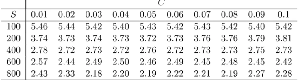
Table 1: Average error rate (%) obtained by polynomial kernels (4.2) with d = 7, L = 3000 C S 0.01 0.02 0.03 0.04 0.05 0.06 0.07 0.08 0.09 0.1 100 5.46 5.44 5.42 5.40 5.43 5.42 5.43 5.42 5.40 5.42 200 3.74 3.73 3.74 3.73 3.72 3.73 3.76 3.76 3.79 3.81 400 2.78 2.72 2.73 2.72 2.76 2.72 2.73 2.73 2.75 2.73 600 2.57 2.44 2.49 2.50 2.46 2.49 2.45 2.48 2.45 2.42 800 2.43 2.33 2.18 2.20 2.19 2.22 2.21 2.19 2.27 2.28
where β and z are variable vectors of size M = 60000 and S, respectively. Thus, the problems have 60000 + S variables with upper and lower bounds, and S + 1 equality constraints. The experiments are conducted on an AlphaServer GS320 workstation (CPU: Alpha21264 1GHz, 4G memory) using CPLEX 7.1 [13] as a linear programming solver.
In Table 1, 2, and 3, we show the test set error rates (%). These tables show the averages over two sampling runs. Table 1 is obtained using the polynomial kernel (4.1) with
d = 7 and L = 3000 sample points. The discriminate functions are generated by solving
the linear programming problem (4.3) with parameter C ranging from 0.01 to 0.1. From Table 1, we observe that the performance is rather insensitive to the choice of parameter
C within this range. Reasonable performance appears to be obtained with C = 0.08.
Therefore, C = 0.08 was used for the rest of our experiments. Table 2 and 3 show the results obtained by the polynomial kernels (4.1) with d = 7 and 8, and those obtained by the RBF kernels (4.2) with γ = 0.2 and 0.4. We sample (L =)1000 or 3000 points out of 60000 training points to extract the subspace FS. The number of dimension S ranges
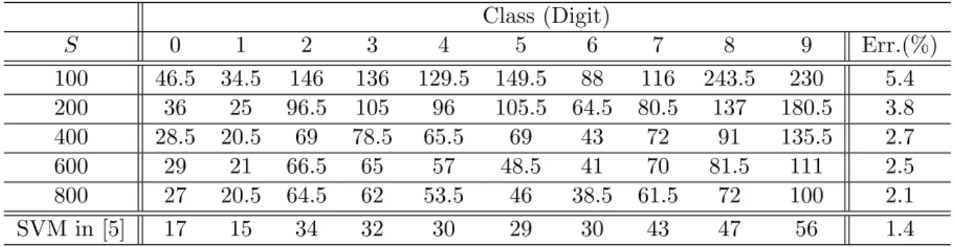
from 100 to 800. In Table 4, we show the total CPU times in seconds for obtaining the discriminate functions for the ten classes. The values in the parentheses indicate the time spent for the eigenvalue decomposition. We solve the same problem using SVMTorch [7], which is one of the commonly used implementations [6] of the standard SVM, and the CPU time is reported in the last row of the table. In Table 5, we show the results of ten binary classifications for each class (digit) obtained using the polynomial kernels with
d = 7, L = 3000 and C = 0.08. The average numbers of test errors out of 10000 test points,
as well as the total error rates (in the last columns), are listed in this table. The last row of the table corresponds to the results of the standard SVM [5] with the polynomial kernel. We see from these tables that both the RBF and polynomial kernels attain around 3% error rates when 400 eigenvectors are used, and that the error rates gradually decrease as the number of eigenvectors increases. Moreover, fairly good performance is achieved by the subspace extracted by a small fraction of the sampled points, which is less than 2% of the entire training set. Table 5 shows that the accuracy of the results obtained by our procedure is slightly less than that for the results in [5] obtained by the standard SVM with the polynomial kernels. However, our discriminate functions are obtained by linear programming, whereas the standard SVM requires quadratic programming.
5. Conclusion
In the present paper, we have proposed a linear programming approach for generating kernel-based nonlinear discriminate functions. The eigenvectors of the Gram matrix are employed to generate the orthonormal basis of the subspace of the feature space F, and the coordinates of the projection of the nonlinearly mapped points φ(x) ∈ F with respect
Table 2: Average error rate (%) obtained by polynomial kernels (4.1), when C = 0.08 d = 7 d = 8 S L = 1000 L = 3000 L = 1000 L = 3000 100 5.67 5.42 5.64 5.42 200 3.99 3.76 4.06 3.75 400 3.17 2.73 3.13 2.74 600 2.56 2.48 2.67 2.39 800 2.49 2.19 2.53 2.24
Table 3: Average error rate (%) obtained by RBF kernels (4.2), when C = 0.08
γ = 0.2 γ = 0.4 S L = 1000 L = 3000 L = 1000 L = 3000 100 5.69 5.46 5.89 5.78 200 4.03 3.84 4.09 3.95 400 3.19 2.78 3.02 2.92 600 2.68 2.43 2.63 2.48 800 2.50 2.22 2.41 2.25
Table 4: CPU time (in seconds)
RBF kernel with γ = 0.2 polynomial kernel with d = 7
S L = 1000 L = 3000 L = 1000 L = 3000 100 857.1 (145.0) 1176.2 (485.5) 798.0 (112.1) 1074.5 (402.9) 200 2064.3 (167.0) 2506.5 (593.7) 1961.8 (133.8) 2263.7 (473.9) 400 7376.4 (311.05) 8367.1 (1017.5) 6634.4 (224.0) 7367.1 (791.4) 600 17312.2 (293.0) 18804.7 (1737.9) 15069.0 (251.8) 15746.9 (1268.2) 800 31927.2 (314.5) 33108.0 (2888.0) 27121.6 (274.9) 27763.7 (2046.6) SVMTorch [7] 75294.9 47988.8
Table 5: Number of errors out of 10000 test points obtained by polynomial kernels with
d = 7 when L = 3000, C = 0.08 Class (Digit) S 0 1 2 3 4 5 6 7 8 9 Err.(%) 100 46.5 34.5 146 136 129.5 149.5 88 116 243.5 230 5.4 200 36 25 96.5 105 96 105.5 64.5 80.5 137 180.5 3.8 400 28.5 20.5 69 78.5 65.5 69 43 72 91 135.5 2.7 600 29 21 66.5 65 57 48.5 41 70 81.5 111 2.5 800 27 20.5 64.5 62 53.5 46 38.5 61.5 72 100 2.1 SVM in [5] 17 15 34 32 30 29 30 43 47 56 1.4
to this basis are explicitly obtained. Through this procedure, we can generate a nonlinear discriminate function by solving a linear programming problem.
We have numerically demonstrated that relatively small dimensional subspace carries enough ability to discriminate between classes. In fact, for the MNIST dataset with 60000 training points, nonlinear discriminate functions of moderate accuracy can be generated in the subspace with 400 dimension. Also, in this setting, our linear programming formulation generates discriminators as efficiently as standard SVMs with the quadratic programming formulation. The proposed procedure takes advantage of the fact that the linear program-ming problem with a large number of variables can be solved when the number of constraints are a few hundred. Moreover, in many practical situations, parameters such as C should be adjusted by performing cross–validation procedures [25], where we need to solve opti-mization problems repeatedly by changing C. In such a situation, a series of several linear programming problems is efficiently optimized by applying the parametric linear program. In addition, since the proposed formulation, as well as the original QPs, has an optimal solution with many zeros, the linear program can be optimized within a smaller number of pivoting iterations. These are the advantages of the proposed method.
Although our computational results are performed using a general purpose linear pro-gramming package as an optimization engine, efficient implementation of a column genera-tion and a chunking method would allow problems to be handled efficiently on PCs. This is a subject for our future research. In addition, the problem for generating multi-class dis-criminators can be handled by extending the proposed linear programming approach, which is now under development.
References
[1] F. Alizadeh and S. Schmieta: Symmetric cones, potential reduction methods and word-by-word extensions. Handbook of Semidefinite Programming (Kluwer Academic Pub-lishers, Boston, MA, 2000), 195–233.
[2] K.P. Bennett and O.L. Mangasarian: Robust linear programming discrimination of two linearly inseparable sets. Optimization Methods and Software 1 (1992) 23–34.
[3] P.S. Bradley and O.L. Mangasarian: Feature selection via concave minimization and support vector machines. 13 th International Conference on Machine Learning (1998), 82–90.
[4] P.S. Bradley and O.L. Mangasarian: Massive data discrimination via linear support vector machines. Optimization Methods and Software 13 (2000) 1–10.
[5] C.J.C. Burges and B. Sch¨olkopf: Improving the accuracy and speed of support vector learning machines. M. Mozer, M. Jordan and T. Petsche eds.: Advances in Neural
Information Processing Systems (MIT Press, Cambridge, MA, 1997), 375–381.
[6] C. Campbell: Kernel methods: a survey of current techniques. Neurocomputing 48 (2002) 63–84.
[7] R. Collobert and S. Bengio: SVMTorch: Support Vector Machines for Large-Scale Regression Problems. Journal of Machine Learning Research 1 (2001) 143–160.
[8] C. Cortes and V. Vapnik: Support-Vector Networks. Machine learning 20 (1995) 273– 297.
[9] N. Cristianini and J. Shawe-Taylor eds.: An Introduction to Support Vector Machines
and Other Kernel–Based Learning Methods (Cambridge University Press, U.K., 2000).
[10] F. Cucker and S. Smale: On the mathematical foundations of learning. Bull. Amer.
[11] S.T. Dumais, J. Platt, D. Heckerman and M. Sahami: Inductive learning algorithms and representations for text categorization. G. Gardarin ed.: 7th International Conference
on Information and Knowledge Discovery (1998), 148–155.
[12] R.A. Horn and C.R. Johnson: Matrix Analysis (Cambridge University Press,
Cambridge-New York, 1985).
[13] ILOG: ILOG CPLEX7.1, user’s manual (ILOG, France, 2001).
[14] T. Joachims: Text categorization with support vector machines: learning with many relevant features. Lecture notes in computer science 1398 (1998) 137–142.
[15] T. Joachims: Making large-scale support vector machine learning practical. B. Sch¨olkopf, C. Burges and A. Smola eds.:Advances in Kernel Methods (The MIT Press, 1999), 169–184.
[16] Y. LeCun, L.D. Jackel, L. Bottou, A. Brunot, C. Cortes, J.S. Denker, H. Drucker, I. Guyon, U.A. M¨uller, E. S¨ackinger, P. Simard and V. Vapnik: Comparison of learn-ing algorithms for handwritten digit recognition. F. Fogelman-Souli´e and P. Gallinari eds.: Proceedings ICANN’95 – International Conference on Artificial Neural Networks (Nanterre, France, 1995), 53–60.
[17] O.L. Mangasarian: Nonlinear Programming (SIAM, Philadelphia, PA, 1994).
[18] O.L. Mangasarian: Generalised support vector machines. A. Smola, P. Bartlett, B. Sch¨olkopf and D. Schuurmans eds.: Advances in Large Margin Classifiers (The MIT Press, 2000), 135–146.
[19] O.L. Mangasarian and D.R. Musicant: Data discrimination via nonlinear generalized support vector machines. M.C. Ferris, O.L. Mangasarian and J.S. Pang eds.:
Com-plementarity : Applications, Algorithms and Extensions (Kluwer Academic Publishers,
The Netherlands, 2001), 233–251.
[20] O.L. Mangasarian, R. Setiono and W.H. Wolberg: Pattern recognition via linear pro-gramming: Theory and application to medical diagnosis. Proceedings of the Workshop
on Large-Scale Numerical Optimization (1990), 22–31.
[21] J.C. Platt: Fast training of support vector machines using sequential minimal optimiza-tion. B. Sch¨olkopf, C. Burges and A. Smola eds.: Advances in Kernel Methods (The MIT Press, 1999), 185–208.
[22] M. Pontil and A. Verri: Support vector machines for 3D object recognition. IEEE
transactions on pattern analysis and machine intelligence 20 (1998) 637–646.
[23] B. Sch¨olkopf, C. Burges and V. Vapnik: Extracting support data for a given task. U.M. Fayyad and R. Uthurusamy eds.: Proceedings, First International Conference on
Knowledge Discovery & Data Mining (1995), 252–257.
[24] B. Sch¨olkopf, A.J. Smola and K. M¨ueller: Kernel principal component analysis. B. Sch¨olkopf, C. Burges and A. Smola eds.: Advances in Kernel Methods (The MIT Press, 1999), 327–352.
[25] M. Stone: Cross–validatory choice and assessment of statistical predictions. Journal of
the Royal Statistical Society 36 (1974) 111–147.
[26] V.N. Vapnik: Statistical Learning Theory (John Wiley & Sons, 1998).
[27] V.N. Vapnik: The Nature of Statistical Learning Theory, (Springer-Verlag, New York, 2000).
[28] J. Weston and C. Watkins: Multi-class Support Vector Machines. Technical Report CSD-TR-98-04, Royal Holloway, University of London, 1998.
Yasutoshi Yajima
Department of Industrial Engineering and Management,
Tokyo Institute of Technology,
Oh-Okayama, Meguro-ku, Tokyo 152-8552, Japan.