Artificial Neural Network based on Simulated Evolution and its Application to Estimation of Landslide

全文

(1)Vol.2011-MPS-83 No.7 2011/5/17. IPSJ SIG Technical Report. learning is large and the error is not necessarily minimized. Moreover, GAs usually take over the configuration of solutions as a scheme of chromosome, the change of values of chromosome is only done by the mutation operator and so, the application of GAs is seemed not appropriate in the application of optimization of parameter values. In this paper, such type of stochastic algorithm as GAs which are based on the evolution of living things is used but Simulated Evolution (SimE) algorithm [2], is newly adopted. Considering this type of value optimization, the steepest descent method in the back propagation process is replaced by SimE algorithm. SimE algorithm has no crossover operator and it only has the mutation operator. This operator is only applied to some of the genes in a chromosome with inferior goodness values. Therefore, SimE algorithm is simple and is expected to be comparatively fast. The ANN with the back propagation using SimE algorithm, called SimE-ANN, is applied to the estimation of landslide [8,9,10] in geotechnical field in order to evaluate its performances by comparing with the conventional steepest descent method. The use of ANN in this study is to predict both displacement and resistance of piles which are used to mitigate landslide hazards in terms of ground movement and instability of slopes. The size of the set of experimental data is 56 and 38 of them are used for training and the remaining 18 data are used for performance evaluations. When comparing with the steepest descent method, the proposed SimE-ANN improves errors of displacement and resistance of the piles 17% and 58%, respectively. The CPU time for the learning is 99% reduced.. Artificial Neural Network based on Simulated Evolution and its Application to Estimation of Landslide Mona Abo-El Dahb†, Yao Zhou†, Umair Farooq Siddiqi† and Yoichi Shiraishi†. The conventional steepest descent method in the back propagation process of an artificial neural network (ANN) is replaced by Simulated Evolution algorithm. This is called SimE-ANN and is applied to the estimation of landslide. In the experimental results, the errors of displacement and resistance of the piles in SimE-ANN, which are the outputs of landslide estimation problem, are 17% and 58% smaller than those of the conventional ANN, respectively. Moreover, the CPU time for the learning is 99% reduced.. 2. Artificial Neural Network 1. Introduction. The operation of ANN depends on the connection between the neuron and the training algorithm.. An artificial neural network (ANN) is considered one of the most widely used tools in the learning processes in various applications [1]. Particularly in supervised learning, the back propagation process is efficient and generally used. In this process, the error between the output of an ANN and the supervised data is propagated backwardly minimizing the error by tuning the parameters of the ANN. Here, such a minimization method as steepest descent method is adopted conventionally but this algorithm tends to be trapped in local minima. Therefore, stochastic algorithms, for example, Genetic Algorithms (GAs) [2], which have hill-climbing ability not be trapped by local minima are applied [3,4,5]. However, in these approaches, all the ANN parameters, for example, the weights of edges and the thresholds of neurons of an ANN are optimized at the same time. As a result, the CPU time needed by †. 2.1 Back Propagation Process The signal flows of this algorithm shown in Figure 1 [1] can be divided into two directions: forward-propagation of information and counter-propagation of error. During the process of forward-propagation, the input information is transmitted into the output layer through the input layer and the hidden layer. If the expected output results cannot be got in the output layer, the error alteration should be worked out. The error signal is counter-transmitted into the neurons in every layer along the primary connection in order to get the expected goal. It makes the input data approach the expected data as quickly as possible. The training process can be over when the sum of the squared errors is lower than the specified value in the output layer. In the end, the weights and the error should be saved.. Department of Production Science and Technology, Gunma University. 1. ⓒ 2011 Information Processing Society of Japan.

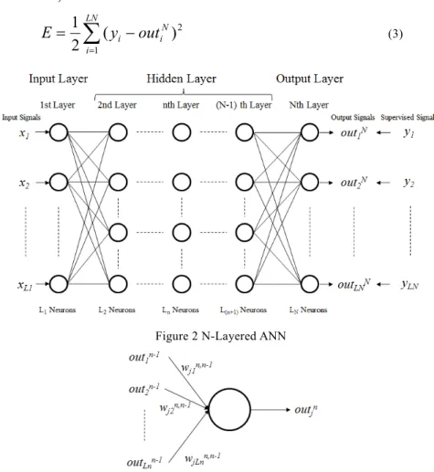
(2) Vol.2011-MPS-83 No.7 2011/5/17. IPSJ SIG Technical Report. the weights. w nji,n−1 , must be minimized during the learning process. E=. 1 LN ∑ ( yi − outiN ) 2 2 i=1. (3). Figure 1 Flow Chart of Back Propagation Process 2.2 Steepest Descent Method Here, an algorithm is needed to minimize the sum of the squared errors by tuning the ANN parameters and, generally, the steepest descent method is used up to now. However, its disadvantage is that the obtained results can often be trapped in a local optimum. The BP with the steepest descent method is described below using the N-layered ANN shown in Figure 2 and the neuron shown in Figure 3. The output of neuron shown in Figure 3 is expressed by the equations (1) and (2).. Figure 2 N-Layered ANN. Ln. net nj = ∑ w nji,n−1out in−1. (1). out nj = f (net nj ). (2). i =1. Here,. net nj. is the input value of j-th neuron in n-th layer and. w nji,n−1. is the weight. assigned to the edge connecting i-th neuron in (n-1)-th layer and j-th neuron in n-th layer. The threshold function f is usually defined as a sigmoid function. The error E which shows the distance of the output of an ANN and the supervised data is defined by the expression (3) as a mean square error. This error E is a function of the output,. out. N i. Figure 3 Configuration of Neuron In minimizing the error E, the steepest descent method is applied. The idea of this method is used in SimE-ANN and so it is explained below. The weight. , which is determined by. w nji,n−1. is changed according to. the expression (4). 2. ⓒ 2011 Information Processing Society of Japan.

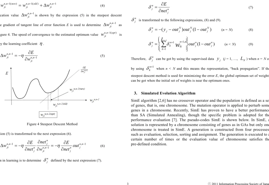
(3) Vol.2011-MPS-83 No.7 2011/5/17. IPSJ SIG Technical Report. w nji,n−1( new) = w nji,n−1( old ) + ∆w nji,n−1 The modification value. ∆w. n ,n −1 is ji. δ jn =. (4). shown by the expression (5) in the steepest descent. method. The gradient of tangent line of error function E is used to determine. ∆w. n ,n −1 ji. as. shown in Figure 4. The speed of convergence to the estimated optimum value. n ,n −1( opt ) ji. is. controlled by the learning coefficient. ∆w nji,n−1 = −η. w. δ nj. ∂E ∂net nj. (7). is transformed to the following expressions, (8) and (9).. δ nj = −( y j − out Nj )out Nj (1 − out Nj )  Ln +1. (n = N). . δ jn =  ∑ δ kn+1 wkj out nj (1 − out nj ). η..  k =1. ∂E ∂w nji,n−1. (5). Therefore, by using. δ nj. δ kn+1. n +1,n. (n < N). . can be got by using the supervised data. yj. (j = 1, …,. (8). (9). LN ) when n = N or. when n < N and this means the representation, “back propagation”. If the. steepest descent method is used for minimizing the error E, the global optimum set of weights can be got when the initial set of weights is near the optimum ones.. 3. Simulated Evolution Algorithm SimE algorithm [2,6] has no crossover operator and the population is defined as a set of genes, that is, one chromosome. The mutation operator is applied to perturb some genes in a chromosome. Recently, SimE has proven to have a better performance than SA (Simulated Annealing), though the specific problem is adopted for the performance evaluation [7]. The pseudo-codes SimE is shown below. In SimE, a solution is represented by a chromosome consisting of genes as in GAs but only one chromosome is treated in SimE. A generation is constructed from four processes, such as evaluation, selection, sorting and assignment. The generation is executed to a certain number of times or the evaluation value of chromosome satisfies the pre-defined condition.. Figure 4 Steepest Descent Method The expression (5) is transformed to the next expression (6).. ∆w nji,n−1 = −η. n ∂E ∂net j ∂E = −η out nj ,n−1 n n ,n −1 n ∂net j ∂w ji ∂net j. The problem in learning is to determine. δ nj. (6). defined by the next expression (7).. 3. ⓒ 2011 Information Processing Society of Japan.

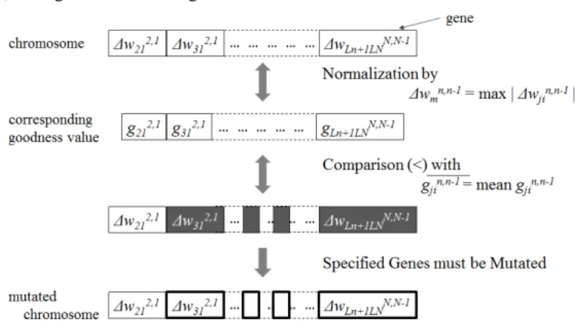
(4) Vol.2011-MPS-83 No.7 2011/5/17. IPSJ SIG Technical Report. algorithm, such genes with small goodness values should be selected.. Figure 5 Outline of SimE processes 4.2 Selection Process The fundamental idea of the selection process is to select such genes with comparatively small goodness values. Therefore, the genes whose goodness values are smaller than the mean value of all goodness values are selected. This selection is done deterministically.. 4. SimE-ANN In the followings, SimE algorithm tailored to optimize the weights of ANN is described. The outline of SimE processes are shown in Figure 5.. 4.3 Allocation Process. As in the expression (6), the value of gene. 4.1 Evaluation Process. A chromosome is defined as a thread consisting of all modification values. ∆w nji,n−1. expression (7). Therefore, the value of. of ANN. shown by expressions (5). The values of genes must be optimized to minimize the error E. The goodness value. g. n ,n −1 ji. corresponding to. ∆w. n ,n −1 ji. ∆w. n ,n −1 ’s. ji. ∆w nji,n−1. δ nj. The. can be freely changed as a real number and so, a range limiter for the new values of. δ nj ‘s is. δ nj. must be. randomly changed to a real number in [ δ j. n. deviation of all. can be regarded as a scale indicating how sensitive. δ nj. 4. − rσ , δ nj + rσ. ‘s and r (r=1, 2 or 3) is a multiplier for. estimation that the values of all. is for changing the error E and the sensitive genes should be mutated. In the SimE. defined by. of selected gene should be controlled. This value. created in order to avoid the divergence. This means that the new value of. goodness values should be used which genes must be selected and mutated in the subsequent. g nji,n−1. be changed by. is defined as the negative. normalized value by the maximum value among all absolute values of. processes. Here, the value. δ nj. ∆w nji,n−1 can. σ. ], where. σ. is the standard. . The value r comes from the. δ nj ‘s would construct a normal distribution and so, it should ⓒ 2011 Information Processing Society of Japan.

(5) Vol.2011-MPS-83 No.7 2011/5/17. IPSJ SIG Technical Report. be determined experimentally. Here, the mutation operator determines the new value of. Table 1 Input and Output Data of Landslide. δ nj. stochastically.. 5. Application of SimE-ANN to Estimation of Landslide This section describes the application of the proposed SimE-ANN to the estimation problem of landslide [8,9,10] to evaluate its performances. Both displacement and resistance of piles are considered the main factors which are responsible for landslide by reducing ground movement and failure. Wakai, et al. obtained a good result by using ANN but this ANN uses the conventional back propagation algorithm. In our study, the actual data got by 3-D FEM are used for evaluating the performances of proposed SimE-ANN comparing with the conventional ANN.. 5.2 Application of Conventional ANN and SimE-ANN To solve the landslide estimation problem, the proposed SimE-ANN is applied and its performances are evaluated against the conventional ANN. The numbers of neurons in the input and the output layers are 8 and 2 and one hidden layer is constructed consisting of 10 neurons. The conventional ANN and SimE-ANN are executed on the computer with 2.33GHz clock frequency and with 2GB main memory. The number of data generated by FEM is 58. 38 of them are used as supervised data for training ANN’s and the remaining 18 are used for testing the ANN’s. The stopping condition of learning process is either of them, the difference of errors between the two successive trainings is less than 0.000001 or the mean square error is less than 0.001. In the steepest descent method, the learning coefficient is set as η=0.1. Here, in SimE, the length of chromosome is 100 and the number of generations is set to 30. The learning coefficient η is 0.001. The value r in the allocation process (5.3) is set to 1 by doing some experiments.. 5.1 Problem Definition The model of landslide [8] is shown in Figure 6. The input and the output data of landslide estimation problem are shown in Table 1. The landslide estimation problem is to generate a pair of data, that is, the displacement of pile heads and the maximum resistance of piles.. 5.3 Errors of Output Both of the ANN’s are tested against 18 test data. The obtained mean square errors are shown in Table 2. As shown in this table, SimE-ANN reduced the mean square errors 17% and 58%, respectively for two outputs, in average.. Table 2 Errors of Conventional ANN and SimE-ANN Figure 6 Model of Landslide. 5. ⓒ 2011 Information Processing Society of Japan.

(6) Vol.2011-MPS-83 No.7 2011/5/17. IPSJ SIG Technical Report. but the CPU time becomes one fifth. SimE-ANN reduced the CPU time 99.17%. The behavior of error values for SimE-ANN is shown in Figure 8(b).. The error values of 18 data are shown in Figure 7 and 18 points are plotted. In these plots, if the output value is equal to the original value, the point is on the 45 degree line. From these plots, it can be seen that the distances between the points and the 45 degree line in SimE-ANN are almost smaller as shown in (b) and (d).. Table 3 Comparison of CPU Time. Figure 8 Comparison of Error Convergences 5.5 Estimated Comparison with Improved BP’s Many improvements have already been done with the original BP [11,12]. The comparison of SimE-ANN with such improved BP’s must be done and this is future work of this research. For the BP with the introduction of entropy term [12], its convergence ratio is evaluated with that of the original BP but their actual processing times are not compared. In the L-BP (BP using the Lyapunov coefficient) [11], the acceleration of the learning process is compared. The examples used in [11] are Exor problem and a simple pattern recognition problem. The sizes and the characteristics of these examples are different from those of landslide estimation problem and so, the exact comparison is inadequate. However, in fact, L-BP reduced the number of trainings (not CPU time) 96% in Exor problem and 98% in a simple pattern recognition problem, respectively. The reduction ratio is almost the same as that of SimE-ANN ((20,991-135)/20,991*100=99.4%). However, the convergence of learning in L-BP is not stable and the authors conclude that the stability of L-BP is not thought better than that of original BP. The convergence of SimE-ANN is guaranteed by the asymptotic optimality of SimE algorithm [2] and it is likely that SimE-ANN attained almost the same ratio of speed up of learning process maintaining the stability of convergence.. Figure 7 Comparison of Errors for Test Data 5.4 Convergence of Error Minimization The CPU times needed for training ANN’s are evaluated. The CPU time of each of the cases is shown in Table 3. The behaviors of error reduction in both of ANN’s are shown in Figure 8. In Figure 8(a), after 20,991 times of trainings, the difference of errors between the two successive trainings is less than 0.000001. Then, the error value is 0.013384 and the required CPU time is 1739.56 seconds as shown in Table 4. Here, the error becomes 3.6 times larger. 6. ⓒ 2011 Information Processing Society of Japan.

(7) Vol.2011-MPS-83 No.7 2011/5/17. IPSJ SIG Technical Report. Journal of the Japan Landslide Society, Vol.42, No.5, pp.18-28 (2006). 9) A. Wakai, S. Gose and K. Ugai: “3-D elasto-plastic finite element analyses of pile foundations subjected to lateral landing”, Soils and Foundations, Vol.39, No.1, pp.97-111 (1999). 10) Akihiko Wakai, Keizo Ugai, and Feng Cai: “Finite element analysis of slopes reinforced with steel piles”, Proc. International Conferences on Slope Engineering, Vol.2, pp.822-827 (2003). 11) Maki Hashimoto, Hirotaka Inoue and Kiroyuki Narihisa: “Stability and Acceleration in the Back Propagation Learning Algorithm”, The Bulletin of the Okayama University of Science, vol.35A, pp.143-152 (1999) (in Japanese). 12) Yutaka Akiyama: “Improvement of the Back-propagation Learning Rule by Introducing an Entropy Term”, IPSJ Transactions on Mathematical Modeling and its Applications, Vol.40, No.SIG9(TOM2), pp.81-90 (1999) (in Japanese).. 6. Conclusions A new artificial neural network based on a stochastic algorithm, called SimE-ANN, is proposed. The implemented stochastic algorithm is Simulated Evolution and this algorithm replaces the conventional steepest descent method in minimizing the error between the output of ANN and the supervised data. The performances of SimE-ANN are evaluated against the conventional ANN for the landslide estimation problem. After trainings for 38 data from 56 data, SimE-ANN reduced the error of displacement of piles and the error of resistance of piles, 17% and 58%, respectively, for the 18 test data. Moreover, the CPU time necessary for the training of SimE-ANN is 99% reduced.. References 1) J. Petrus: “Artificial Neural Networks, An Introduction To ANN Theory and Practice”, Springer (1995). 2) Sadiq M. Sait and Habib Youssef: “Iterative Computer Algorithms with Applications in Engineering”, IEEE Computer Society Press (1999). 3) David Montana and Lawrence Davis: “Training feedforward neural networks using genetic algorithms”, in Proceedings of the 11th International Joint Conference on Artificial Intelligence, pp.762-767, Morgan Kaufmann (1989). 4) Daniel Rivero, Julian Dorado, Enrique Fernández-Blanco, and Alejandro Pazos: “A Genetic Algorithm for ANN Design, Training and Simplification”, J. Cabestany et al. (Eds.): IWANN 2009, Part I, LNCS 5517, pp.391-398 (2009). 5) WenFeng Feng, WenJuan Zhu, and YuGuang Zhou: “The Application of Genetic Algorithm and Neural Network in Construction Cost Estimate”, Proceedings of the Third International Symposium on Electronic Commerce and Security Workshops (ISECS ’10), Guangzhou, P. R. China, 29-31, pp.151-155, July (2010). 6) H. M. Kling and P. Banerjee: “Concurrent ESP: A placement algorithm for execution on distributed processors”, Proc. of the IEEE International Conference on Computer-Aided Design, pp.354-357 (1987). 7) Umair F. Siddiqi, Yoichi Shiraishi, Mona A. El-Dahb and Sadiq M.Sait, "Embedded Systems Synthesis Using Simulated Evolution (SimE) with ECU-Specific Optimization", Proceedings of International Conference on Computer Mathematics and Natural Computing, ICCMNC 2011, Penang, Malaysia, February (2011). 8) Akihiko Wakai, Keizo Ugai, Fei Cai and Kiyoshi Tanaka: “Simple computer-aided design system for rational evaluation of maximum resistance of landslide prevention piles”, 7. ⓒ 2011 Information Processing Society of Japan.

(8)