著者
ZHANG Changping
雑誌名
国際地域学研究
巻
-号
15
ページ
85-97
発行年
2012-03
URL
http://id.nii.ac.jp/1060/00003664/
Creative Commons : 表示 - 非営利 - 改変禁止 http://creativecommons.org/licenses/by-nc-nd/3.0/deed.jaSpatial Weights Matrix and its Application
Changping ZHANG
1 Introduction
A spatial weights matrix W what is indicates the strength of the potential interaction between spatial areal units. The choice of W is a critical step in spatial analysis and can influence the significance of testing procedures (Tiefelsdorf, Griffith, and Boots, 1999). To think about the type of spatial weights matrix W, Getis (2009) indicated that at least three ways exist that could be theoretical, topological, and empirical points of view. According to theoretical point of view, the W matrix is exogenous to any system, and should be based on a preconceived matrix structure. Usually this structure is based on a theory of distance decay, however defined. The theory of distance may come from notions of spatial interaction and gravity models. The topological viewpoint arose from a need to depict the actual configuration of the areal units contained within a study region. For example, a long, narrow areal unit would be represented in differently than a short, wide unit. In this case the matrix W might be specified in different ways that might be number of neighbors, length of side in common, and proportion of perimeter in common. Cliff and Ord (1969) said, “With a flexible system of weights, the researcher can highlight those features of a study area which he believes to be important”. The empirical viewpoint of approach implies that one detects spatial dependence in variables under study. One must use a local autocorrelation point of view to identify the exact level of spatial autocorrelation surrounding any given observation then creates a W matrix.
Since 1960s, most researchers have made every effort to attempt to create proper dependence representation in spatial weights matrix W. When data are in a raster model, W was constructed in the rook’s case or queen’s case definition of neighbors. Using vector data, popular were two types of W to be used. The first is called a simple binary connectivity definition and uses a discrete function where spatial entities are assumed to be adjacent if and only if they share a common boundary. The nature of interaction for the spatial phenomenon under study cannot always be captured by a simple binary proximity measurement. In this case, based on theoretical and conceptual considerations, a generalized weight function can be used as advanced by Cliff and Ord (1981) which offers flexibility in defining spatial proximity. Typical functions incorporate the distance between the geographical centroids of areal units and / or the length of common boundary between areal units (Can, 1996).
Getis and Aldstadt (2004) summarized previous attempts to create a spatial weights matrix and identified many different types of weighting schemes. That are
1. spatially contiguous neighbors;
2. inverse distances raised to some power;
3. length of shared borders divided by the perimeter; 4. bandwidth as the nth nearest neighbor distance; 5. ranked distances;
6. constrained weights for an observation equal to some constant; 7. all centroids within distance d; and
8. n nearest neighbors, and so on Some of the newer schemes are: 1. bandwidth distance decay; 2. Gaussian distance decline; and 3. “tri-cube” distance decline function.
Furthermore, Getis and Aldstadt (2004) also proposed a spatial weights matrix based on the Gi* local
statistic (Ord and Getis, 1995) which accounts for the spatial association extant within any region that has been divided into its constituent parts. In a series of simulation experiments the matrix is compared to well-known spatial weights matrix specifications - two different contiguity configurations, three different inverse distance formulations, and three semi-variance models and performed best according to the AIC (Akaike Information Criterion) and the autocorrelation coefficient evaluation.
Zhang and Murayama (2000) suggested a concept and algorithm of k-order neighbours based on Delaunay’s triangulated irregular networks (TIN) and redefined Getis & Ord’s (1992) local spatial autocorrelation statistic as Gi (k) with weight coefficient wij (k) based on k-order neighbours for the study of
local patterns in spatial attributes.
Although the choice of a spatial weights matrix specification for spatial statistical analysis is not clear-cut and seems to be governed primarily by convenience or convention, Griffith (1996) proposed some explicit guidelines on specification of the spatial weights matrix and concluded that relative large numbers of areal units should be employed (n > 60) in a spatial statistical analysis and low-order spatial models should be given preference over higher-order ones.
2 Definitions of spatial weights matrix
In this section, four types of weight coefficient are defined and the spatial weight matrices formed by these coefficients are created for a simple hypothetical region.
2.1 Binary weight
If we are studying spatial interrelationships distributed over a set of areal units, the spatial structure of units might be defined as the spatial contiguity which is treated as a n×n spatial weights matrix W with
binary variable (Cliff & Ord, 1981; Zhang and Murayama, 2003). The binary weight is represented as follows: = otherwise. 0 ; contiguous are and area if 1 j i wij (1)
The binary spatial weights matrixW is a symmetric form. If the W is row-standardized:
∑
∈=
J j ij ij * ijw
w
w
where J is the set which includes all areal units that are contiguous with i. the wij* is satisfying non-negative
wij*≧0 and
∑
*=
1
∈J
j ij
w
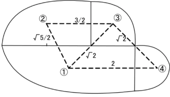
(for all i = 1, … , n). The binary weight is often used in spatial autocorrelation analysis with regular and irregular areal units. A hypothetical example will clarify the use of this index. Imagine a region that is divided into four units (Figure 1), unit 1 and 2, 1 and 3, 1 and 4, 2 and 3 are contiguous. ① ② ③ ④ √2 √2 2 √5/2 3/2Figure 1. A hypothetical region
The binary spatial weights matrix and its standardized form of figure 1 are
=
0
0
0
1
0
0
1
1
0
1
0
1
1
1
1
0
bW
=
0
0
0
1
0
0
5
.
0
5
.
0
0
5
.
0
0
5
.
0
3333
.
0
3333
.
0
3333
.
0
0
* bW
2.2 Distance decay weight
Tobler (1970) has referred to as the “first law of geography: everything is related to everything else, but near things are more related than distant things.” In researches on the interrelation and interaction, the phenomenon in which the contiguity or interaction will decrease with increasing distance between two areal units is called as distance decay. The distance decay weight is usually expressed as a reciprocal of distance.
ij ij
d
w
=
1
(2)where dij is the distance from the center of units i to the neighboring units j. Generally the distance can be
straight-line distance, road distance, time distance, cost distance, mental distance, or some other way. The distance decay spatial weights matrix and its standardized form of figure 1 are
=
0
2
1
29
2
2
1
2
1
0
3
2
2
1
29
2
3
2
0
5
2
2
1
2
1
5
2
0
dW
=
0
4480
.
0
2353
.
0
3168
.
0
3398
.
0
0
3204
.
0
3398
.
0
1923
.
0
3450
.
0
0
4628
.
0
2379
.
0
3365
.
0
4256
.
0
0
* dW
2.3 Generalized weightA generalized weight definition based on distance and length of boundary between areal units. In this case, the elements of spatial weights matrix W are:
∑
∈=
J j ij ij ij ijd
l
l
w
(i = 1,…, n) (3)where J is the set which includes all units that are contiguous with unit i. lij is the length of join between
units i and j.
∑
∈J
j ij
l
is the length of all joins for unit i, i.e. its perimeter; and dij is the distance from the centerof units i to the neighboring units j.
∑
∈J j ij ijl
l
is simply the proportion of the perimeter of unit i which is contiguous with unit j. This weighting function assumes that the interaction between two units will increase with increasing length of common boundary and will decrease with increasing distance between their geographical centers. The generalized spatial weights matrix and its standardized form of figure 1 are
=
0
0
0
2
1
0
0
3
1
2
2
1
0
9
2
0
5
3
4
8
1
2
4
1
5
1
0
gW
=
0
0
0
0000
.
1
0
0
4852
.
0
5148
.
0
0
2715
.
0
0
7285
.
0
1669
.
0
2360
.
0
5971
.
0
0
* gW
2.4 k-order neighbors weight
Zhang and Murayama (2000) proposed a concept of k -order neighbors based on Delaunay’s triangulated irregular network (TIN) with centroids of areal units and a definition of k-order neighbors weight. For example, figure 2(B) shows the result of drawing a TIN based on the point distribution in figure 2(A). The k-order neighbors in the Delaunay triangulation network are defined as follows. Those points directly connected to a point v by the edges of the TIN are called the "nearest neighbors", or "1-order neighbors" of this point (figure 2 (C)). Then, those points which are directly connected to the first-order neighbors, of that are not 1-order neighbors themselves, are called "2-order neighbors" (figure 2 (D)). By continuing this process we can define k-order neighbors for any point, v.
The weight coefficient wij (k), which measures proximity of k-order neighbors in a point distribution, is
determined as follows. wij (k) is binary coefficient set to 1 if point j is a k-order neighbour of point i,
otherwise, it is 0. Hence, = otherwise. 0 ; point of neighbour order -a is point 1 ) ( i k j k wij (4)
# # # # # # # # # # # # # # # # # # # # # # # # # # # # # # # # # # # # # # # # # # # # # # # # # # # # # # # 0 1 2 3 4 5 6 0 1 2 3 4 5 6 7 8 9 10 11 12 13 14 15 16 17 18 19 20 21 B C D A
Figure 2. k-order neighbors based on Delaunay triangulation. (A) point distribution, (B) Delaunay triangulation, (C) nearest neighbors, (D) 2-order neighbors.
The 1-order neighbors spatial weights matrix and its standardized form of figure 1 are
=
0
1
0
1
1
0
1
1
0
1
0
1
1
1
1
0
kW
=
0
5
.
0
0
5
.
0
3333
.
0
0
3333
.
0
3333
.
0
0
5
.
0
0
5
.
0
3333
.
0
3333
.
0
3333
.
0
0
* kW
3 Prominence of areal units
In spatial statistical analysis of geographical phenomena, a region or a city under study might be divided into some small areal units such as a regular square tessellation or administrate units emerged in irregular shape and have different spatial characteristics. If we are using GIS to support the analysis, irregular areal unit such as cho in Japan is usually represented as one such polygon with geometric attributes. In spatial statistics, an areal unit that has special geometric attributes and maintains significant spatial correlation and spatial interaction close to adjacent units is called a prominent areal unit or important areal unit. The prominence of areal units can be measured by a prominence or influence-centrality index which is obtained by using eigenfunction or Markov chains method from a spatial weights matrix (Tinkler, 1972; Griffith and Jones, 1980; Boots, 1982; Bavaud, 1998, Zhang and Murayama, 2003).
In this Study, we will use four types of weight function definition to create different measures of prominent areal units and use them to analyze the urban spatial pattern in Matsudo City, Chiba Prefecture.
3.1 Eigenfunctions method
In several geographical literatures it is suggested that the principal eigenvector can be used to measure the prominence of irregular areal units (Tinkler, 1972; Griffith and Jones, 1980; Boots, 1982). The eigenfunctions of spatial weights matrix is
(
)
0
det
)
(
0=
=
−
=
− =∑
n n i i ia
W
I
λ
λ
λ
φ
(5)The eigenvalues are the roots of W. Since spatial weights matrix W is real, the λi are real and may be
ordered as λ1≧…≧λn . Corresponding to each λi is an eigenvector vi , which satisfies
i i
i
v
Wv
=
λ
(i = 1, 2, …, n) (6)The elements of v1 corresponding the largest eigenvalue λ1 provide a measure of the relative position of
each areal units since the magnitude of the element is related to the centrality or prominence. Generally, a unit located in central region of a city possesses a larger element of v1, vice versa a unit with smaller element
might be located near the city limit.
3.2 Markov Chains method
The standardized spatial weights matrix W * with elements of row-standardized variable wij* is identical
to the Markov chains transition matrix. Assuming the chain is ergodic (
(
w
n)
ij>
0
for some n(> 0)and all i, j ), we can obtain a unique stationary distributionp
j>
0
, (∑
jpj =1.0) solution:p
p
W
T=
(7) or ij j jpjw = p∑
The vector p, pT =(p L1, pn)is an eigenvector of WTwith a corresponding eigenvalue of 1. Whereas w
ij
is a measure of the relative influence of unit j on unit i, pi can be interpreted as the total influence of unit i
on the total region of city. pi will be further referred to as a prominence index (Bavaud, 1998). We also call
the index as spatial prominence pi here because the spatial attributes are necessary to calculate it.
3.3 Examples
As mentioned above, different prominences can obtained from different spatial weight matrices. We use the standardized spatial weight matrices to calculate the prominence of units of figure 1. The elements of eignvector p of binary spatial weights matrix Wb* are
p1 = 0.375, p2 = 0.250, p3 = 0.250, p4 = 0.125.
Areal unit 1 has the largest value of prominence, because it is contiguous to three other units. The prominence of unit 2 is just the same value as unit 3, because they are all contiguous to two units. As the unit 4 is only contiguous to unit 1, it has the least prominence.
The elements of eignvector p of distance decay Wd* are
p1 = 0.273, p2 = 0.251, p3 = 0.270, p4 = 0.205.
The value of prominence of unit 1 is similar unit 3, because their distances linked to other units are almost equivalent. The prominences of unit 2 and unit 4 are all smaller than unit 1 and unit 3 since they are quite separate from each other. As unit 2 is nearer to unit 1 than unit 4, its prominence is larger than unit 4.
The elements of eignvector p of generated Wg* are
p1 = 0.409, p2 = 0.335, p3 = 0.188, p4 = 0.068.
Areal unit 1 has the largest value of prominence, because it possesses the largest unit and longest common boundary joined with other units. The prominence of unit 2 is larger than unit 3 since unit 2 has a longer boundary and a shorter distance joined to unit 1 than unit 3. The prominence of unit 4 is smallest within 4 units.
The elements of p of 1-order neighbors Wk* are
p1 = 0.3, p2 = 0.2, p3 = 0.3, p4 = 0.2.
As unit 1 and unit 3 are all directly connected to other 3 units by the edges of the TIN, their prominences are same as 0.3. Similarly, unit 2 and unit 4 are all only connected to other 2 unit, their prominences are smaller than unit 1 and unit 3 as same as 0.2. Therefore, the variation of prominence based on 1-order neighbors weight is relatively smaller and its sensitivity is lower comparing with other types of weight.
As a result of above analysis, the variation of prominence of areal units is depending on the definitions of spatial weights matrix. The binary weight is affected by the topological attributes and the generated weight is impacted by the geometric attributes. The distance decay is completely determined by the distance between tow units. However the influence of geometric attributes is not definitely reflected in 1-order neighbors weight .
4 Application
Matsudo is a midsize city located in north-eastern part of Tokyo metropolitan area. Its administrative division was formed when the municipality was established in 1953. The cho is the fundamental administrative areal unit and the variation of its geometric attributes is very large. For example, the area of the biggest cho is 185 times as large as the smallest, and the longest distance from the center of a cho to the neighboring cho is 22 times as long as the shortest.
The standardized binary, generated, distance dancay and 1-order neighbors spatial weight matrices Wb*,
Wd*, Wg*, Wk* can be derived from topological attributes of the polygons of chos and TIN data which are built by GIS e.g. ArcGIS and digital map 2500 constructed by Japanese Geographical Survey Institute (Can, 1996; Zhang, 1999; Zhang and Murayama, 2000). Then the spatial prominences pi can be calculated
according to the equation (7). Figure 3 shows 4 distributions maps of classified prominence of chos in Matsudo city.
We can consider Figure 3(A), which shows that the prominent chos with larger than 0.006 of pi are
concentrated on the triangular region formed by the eastern side along the JR Jouban Train Line, the western side along the JR Musashino Train Line, and the northern and southern sides along the Keisei Subway Line. There are a large number of large and non-compact chos in the region. In contrast, small and compact chos show lower value of prominence and are located on the periphery of Matsudo city.
Figure 3(B) shows a distribution map of the prominence based on distance decay weight. As shown in this figure, chos with larger than 0.004 of pi tend to be concentrated in central region and the northern region
of the city. There are many small chos with relatively regular shape. In reverse, many larger chos with less than 0.004 of pi are distributed in the southern and western parts of the periphery of the city. The distribution
(A) Binary (B) Distance decay
(C) Generated (D) 1-order neighbour
Figure 3. Prominence distributions in Matsudo city
The distribution of prominence based on generated weight of chos is represented in figure 3(C), and it can be seen that chos with larger prominence value are distributed along the main train lines in which a lot of large and non-compact chos are located. Reversely, in the region with smaller prominence value, a lot of small chos with relatively regular shape are located there. Another wide region with smaller prominence value is located at southern sides along the Keisei Subway Line.
As can seen from distribution of prominence based on 1-order neighbors weight (figure 3(D)), some clustered regions are not formed and chos with different value of prominence are widely distributed in entire
Matsudo city.
5 Conclusion and future prospects
In regional science, an areal unit which has special geometric attributes and keeps significant spatial correlation and spatial interaction closely to adjacent units is called prominent zone. The prominence of irregular units can be measured by prominence index which is a stationary distribution of Markov chains transition matrix identical to a spatial weight matrix.
In this study, to identify the strength of the potential interaction and correlation between spatial units, we reviewed previous researches to create the spatial weights matrix and discussed some explicit guidelines on specification of the spatial weights matrix and many different types of weighting schemes. Then four definitions of spatial weights are showed as binary, distance decay, generalized, and k -order neighbors weight and prominences are obtained form these weights matrix. Finally we used them to analyze the spatial pattern in Matsudo City. The result of this analysis is shown as though different prominences can get from different weights matrix, generalized weight matrix is more appropriate to measure prominence of units than the distance decay and k-order.
As we know that the spatial structure of city is determined by not only geometric attributes and topological attributes, but also social and economic thematic attributes of areal units in city, it is necessary to create some definitions and measures for prominent unit and to use them to analyze the urban spatial structure. The definitions propose begin with confirming the relationship between the prominence index and geometric attributes of areas, expand to include all spatial attributes of areas: geometric attributes, topological attributes and thematic attributes. Furthermore, an approach to implement the definitions will be tested and evaluated to analyze the spatial structure of a city.
References
Bavaud, F. (1998). Models for spatial weights: a systematic look. Geographical Analysis, 30, 153-171.
Boots, B. N. (1982). Comments on the use of eigenfunctions to measure structural properties of geographic networks.
Environment and Planning, A 14, 1063-1072.
Can, A. (1996). Weight matrices and spatial autocorrelation statistics using a topological vector data model. International
Journal of Geographical Information Systems, 10, 1009-1017.
Cliff, A. D. and Ord, J. K. (1981). Spatial processes: Models and applications. London: Pion.
Cliff, A. D. and Ord, J. K. (1969). The problemof spatial autocorrelation. In A. J. Scott (Ed.) London Papers in Regional
Science, Volume 1, Studies in Regional Science (pp. 25-55). London: Pion.
Getis, A. (2009). Spatial weights matrices. Geographical Analysis, 41, 404-410.
Getis, A. and Aldstadt, J. (2004). Constructing the spatial weights matrix using a local statistic. Geographical Analysis, 36, 90 -104.
-206.
Griffith, D. A. and Jones, K. G. (1980). Explorations in the relationship between spatial structure and spatial interaction.
Environment and Planning A, 12, 187-201.
Griffith, D. A. (1996). Some guidelines for specifying the geographic weights matrix contained in spatial statistical models. In S. L. Arlinghaus et al. (Eds.) Practical Handbook of Spatial Statistics (pp.65-82). Boca Raton: CRC.
Ord, J. and Getis, A. (1995). Local spatial autocorrelation statistics: Distributional issues and an application. Geographical
Analysis 27, 286-306.
Tiefelsdorf, M., D. A. Griffith, and B. Boots, (1999). A variance-stabilizing coding scheme for spatial link matrices.
Environment and Planning A, 31, 165-180.
Tinkler, K. J. (1972). The physical interpretation of eigenfunctions of dichotomous matrices. Transactions of the Institute of
British Geographers, 55, 17-46.
Tobler, W. R. (1970). A computer movie simulating urban growth in the Detroit region. Economic Geography, 46 (Supplement), 234-240.
Zhang, C. (1999). Development of a spatial analysis tool for irregular zone using the spatial data framework. Geographical
Review of Japan, 72, 166-177. (in Japanese with English abstract)
Zhang, C. and Murayama, Y. (2000). Testing local spatial autocorrelation using k-order neighbors. International Journal of
Geographical Information Science, 14, 681-692.
Zhang, C. and Murayama, Y. (2003). Evaluation on the Prominences of Irregular Areas Based on Spatial Weight Matrices.