Hyperexponential Waiting Time Structure in Hyperexponential HK/HL/1 Systems

Journal of the Operations Research Society of Japan

Vol. 28, No. 3, September 1985

HYPEREXPONENTIAL WAITING TIME STRUCTURE

IN HYPEREXPONENTIAL

HK/HL/l

SYSTEMS

Julian Keilson

The University of Rochester

Fumiaki Machihara

NIT Musashino Electrical Communication Laboratories

(Received November 21,1984: Revised April 19, 1985)

Abstract Elementary congestion models sometimes require analysis of G/G/l systems with hypere.xponentially distributed interarrival time and service time distributions. It is shown that for such systems, the ergodic waiting time distribution is itself hypere.xponentially distributed. A simple computational procedure is provided to fmd the parameters needed. Green's function methods are employed to motivate the factorization required. The relevance of these results to the delay in the overflow process of M/M/S is discussed.

1. Introduction. The Lindley Process

Let HK be the class of hyperexponential variates of order K, i.e. of variates which are a mixture of K distinct exponential variates. In an HK~L/l queue, a sequence of cust~mers C

K arrive at a single-server queue at epochs 'k' The interarrival times ~k

=

'k+l - 'k are i.i.d. with p.d.f. f~(x)

=

K

-A

.x

I

a.A.e ] (A <A <····<A). The service times TK also form an i.i.d. sequence

j=l ] ] 1 2 K

L -1-I.X with p.d.f. fT(x)

=

L

b.1-I.e ~ (1-I

1<1-I2<····<1-IL). If Xk is the time that the

i=l ~ ~

k-th customer must wait in queue for service, then X

k+1 max [0, Xk+~k+l]

where ~k+l

=

Tk-~k' The process

x

k is called the Lindley waiting time process

[6]. In this paper, the ergodic Lindley waiting time distribution is shown to be itself hyperexponential in density of order L apart from the mass point at the origin. To establish this result, Green's function methods are employed

[2]. The hyperexponential structure is then obtained by complex plane argu-ments. Comparable results have been exhibited for M/HL/l systems previously

[4]. The extension to H /H /l, however, is non-trivial and suggests that the © 1985 The Operations Research Society of Japan

exponential spectra obtained for HK/HL/l might carry over for other system variates of interest such as the busy period.

It is known that for an M/M/S queue with finite storage, the overflow process has intervals between departures which are independent and of hyper-exponential distribution [7]. For a switching system in which the overflO1. stream is routed to a single server with hyperexponentially distributed

service, the results exhibited may have practical value. The results may also be of interest elsewhere in congestion theory.

2. The Green I s Function for the Underlyiing Homogeneous Process

I t is assumed that the reader is familiar with Green's function methods and the idea of compensation. A simple short presentation may be found in [1] where other references are given. Other details may be found in (2].

It is shown in [3] that the ergodic Lindley waiting time distribution has a generalized density function foo(x) which may be expressed in terms of th': ergodic Green density goo(x) of the underl.ying spatially homogeneous random walk and the compensation density coo(x) representing the influence of the boundary at x=O. The ergodic Green density is given by

8(x) +

I

ain) (x) n=l k

(2.1) g (x)

00

where 8(x) is the delta function for unit mass at 0 and

a€~)(x)

is the n-fold convolution of the p.d.f. of ~k' The generalized compensation density coo(x)

has a delta function component of positive mass cooO at x=O and a negative density distributed on (-oo, 0) with mass equal to -cooO so that the total com-pensation mass is zero. One then has as stated

(2.2) f 00 (x) =

Joo

c co (x') g co (x-x' ) dx' •

-00

The structure of goo(x) will be studied in this section through its Laplace transform (2.3) -5~k where a~ (5) = E[e ]. k

I

a~

(5) n=O k l/(l-a~ (5» k

Hereafter we write ~ instead of ~k for simplicity. From the definition of ~, since ~ ,= Tk -f',k' one has

244 J. Keilson and F. Machihara

(2.4)

K A. L ]Ji

( La.

~)

( Lb. --).

j=1 J I\j-S i=1 ~ ]Ji+s

A . ]J . A .]J . 1 1 Since J ~ J ~ ( _ _ + _ _ )

A .-s jJ.+s

=

A .+jJ. A .-s ]J.+s'

] ~ J ~ J ~

E[e-s~] can be written as

(2.5) where

(2.6) 1, p., q.>O for all j=l, 2, ... , K and

J ~

=1, 2, ••. , L.

From (2.3), (2.5) and (2.6) one then finds

(2.7) L {goo (x) } K A. L _]Ji K p. L _qi 1- \' p. _J __

_L

_{q. s[}

_L

_J_+

_L

]J

.+~;]

'" J A -s ]J.+s S-A. j=1 j i=1 ~ ~ j=1 J i=1 ~ Let (2.8) x(S) Then K Pj

- L

(S-A.)2 j=1 ] L qi

L

(]J.+s)2 < 0 for all real values of S which are

.i=1 ~

not poles.

I t follows that x(s) has one simple zero between adjacent poles. I f the ergodity condition E[lI

k]'-E[Tk]>O is satisfied, one has from (2.8)

(2.9)

Equation (2.9) shows that x(s) has one zero between the first negative pole and zero (See Figure 2.1). Hence, the number of negative zeros is equal to L and the number of positive zeros is equal to K-l.

(N) (N)

positive zeros respectively be denoted by -SI ,-s2 '

••• <

-siN)

<

-s;N))

and

s~P),

siP), ... ,

s;~~

Let the negative (N)

.... , -sL

(r(p) < rep) <:

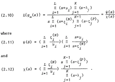
"1 "2 With this notation, (2.7) can be recast into the form

(2.10) where (2.11) 1jJ(S) and (2.12) X (s) L K IT (s+P.) IT (s-A.) i=l ~ j=l ) L K-1 s IT

(s+~~N»

IT

(s-~~P»

i=l ~ j=l ] (N) L ~. L S+ll . IT -~-)( IT

(~»

i=l lli i=l s+~ .

~ K-1 L

~~N)

s IT ( s-

~ ~p

) ) ( IT -~ ) j=l ] i=l lli K IT (s-A.) j=l ] 1jJ(s) = X (s)

I t should be noted that the following inequality is satisfied:

(2.13) < •••• < x(s) A I 21 I 1

246 J. Keilson and F. Machihara

3. The Ergodic Waiting Time Distribution

The following factorization theorem for Green's function goo(x) may be employed:

Theorem.

Let i;=T-!::., where T and!::. are independent non-lattice random variables with finite first moments and E(T)-E(L'I)<O. Let R={s:Res::;:O} and

L={s:Res~O}.

Then {l_E[e-si;]}-l may be written uniquely as a ratio

for which

a) ~oo(s) is regular inside R, and uniformly bounded and non-vanishing on

R;

b) Xoo(s) is regular inside L and non-vanishing in the interior of L with a simple zero at s=O;

c) ~ (0+ )=1.

00

Proof:

This theorem is a variant of similar factorization theorems for Hilbert problems [8]. The non-vanishing of ~oo(s) is discussed in [5] in the context of the Spitzer identity. The non-vanishing of Xoo(s) arises from the structure of the compensation measure and is equivalent to the statement that

-sx

for any non-positive, non-lattice variate

x,

X(s)=E[e ] has the value 1 on L only at s=O. The uniqueness is as usual obtained from Liouville's Theorem. Thus i f we had distinct function pairs ~1 (s), Xl (s) and ~2 (s), X

2 (s) with the properties stated, we would have {~1(s)/~2(s)}={Xl(s)/X2(s)} on the imaginary axis. Each expression in eurly brackets is regular and uniformly bounded in its half-plane, etc. Note that E[T]<E[!::.] assures that X

1(s) and X2(s) have a simple zero at s=O so that the ratio X

1(s)/X2(s) is bounded near s=O. Each expression must then be constant and the uniqueness follows.

By examination of (2.10) we verify that ~(s) and x(s) given by (2.11) and (2.12) have the desired properties. Therefore, ~(s) is the Laplace transform of the ergodic Lindley waiting time density function foo(x). ~(s) can be written as

L r,. (N) L r,~N)

(3.2) ~(s) IT -~-)(1 +

LW.

] )

i=l ]J. . ~ j=l ] s+r,\N) ]

where

and

W.

]

I t is clear from (2.13) that 10'1 >0. From -r;;

~N)

+ll <0 and -r;;

~N)

+r;; (N) <0 for

] k ] k

j-1 j-1

k=l, 2, .•. , j-1, one has IT

(-r;;~N)+ll

)/ IT

(_r;;~N)+r;;(N»>o.

Noting that

k=l ] k k=l ] k _ (N) > _ . _ (N) (N)

r;;j +llk 0 k-), ••• , Land r;;j +r;;k >0, k=j+1, ••• , L, one has wj>O.

The inverse transform of (3.2) gives

(3.3) where f _co() = L r;;~N) IT -~­ i=l lli From (3.3) we have

for the survival function

F

(x)

=

p[x

>x] of the ergodic waiting time

00 00 (3.4)

F

(x) 00 L (N)

L

fco()",.exp(-r;;. x), j=l ] ] x>O.

To obtain

foo(x)

and

F

(x)

numerically WE! only need the zeros

r;;~N).

These are

00 ]

easily obtained to great accuracy from (2.13) by standard bisection methods. I t follows that

foo(x)

and

Foo(X)

are hyperexponential functions of order

L

apart from the mass point at the origin.

4. Structure of the Green's Function and Compensation Density

From (2.10) one then obtains the following explicit form for

goo(x)

away from the origin, at which point

goo(x)

has a delta function representing its mass point. One has

248 J. Keilson and F. Machihara L (N)

I

p.exp(-~. x), x>O i=1 ~ ~ (4.1) 'I K-l (p)

~-E(T

) -

.I

8.exp(~.

x) , k k J=1 J J x<O ,

where as may be seen from (2.7)

and -8. J L IT (_~(N)+)J ) k=1 1 k L IT (_r(N)H(N)) " I ' k k=2 j

=

2, 3, ... , L j (p) K IT (~. _{-Ak )} IT «P)-A) k=1 J k=j+l ~j k j = 2, 3,

...

,

K-l.

From (2.13) one can easily find p .>0 for j=l, 2, ... , Land 8.>0 for j=l, 2,

J J

••• , K-l.

From (2.2), (4.1) and properties of the compensation density, 0+ f (x)

=

f

C (x')g (x-x')dx' 00 00 00 -00 (4.2) L (N) 0- (N)

I

p.exp(-~. x)[/ C (x')exp(~. x')dx'+cooQ]' x>O.

o-Noting that

f

C (x')dx'+c

'" "'0 0, c(x')SO for all x'<O and

exp(t~N)x')<l

~ for

all x'<O, one has

o-f

c

(x')exp(t~N)x')dX'+c

> 0 " ' . ~ " ' 0 '

I t then follows that f",(x) is a hyperexponential function of order L on (0, co). This assures the result of Sec. 3. The hyperexponentiality of

{E[~]}-l_g (x)

_00. of order K-1 on (-co, 0) is obtained in the same way.

The compensation density cco(x) for negative x can be written as [2, pp. 104-108] .

(4.3) -fcoas(x-y)fco(y)dY,

o

x<O .

From (2.5) and (3.3), one has

c _co (x)

-J { I

co K p.A.exp(A.(X-X'»}{

I

L fcoOw.t.N exp(-t.( ) ( ) N x')dx'}

o

j= 1 ] ] ] i= 1 ~ ~ ~

(4.4)

x<O .

References

[1] Graves, S. C. and Keilson, J.: "The Compensation Method Applied to a One-Product Production/Inventory Problem," Mathematics of Operations

Research, 6, 2 (1981), pp. 246-262.

[2] Keilson, J.: Green's Function Method in Probability Theory, Charles Griffin and Company, London (1965)

[3] Ke i 1 son, J.: "The Ro le 0 f Green' s ~unc t ion in Conge s t ion Theory," l'roc.

Symp. on Congestion Theory, University of North Carolina Press (1965), pp.43-71.

[4] Keilson, J.: "Exponential Spectra as a Tool for the Study of Server Systems with Several Classes of Customers," J. of Appl. Prob. 15 (1978), pp.162-170.

[5J Kingman, J. F. D.: "The Heavy Traffic Approximation in the Theory of Queues, Discussion by Keilson J.", Pro~. Symp. on Congestion Theory, University of North Carolina Press (1965), pp.162-164.

Cam-250 J. Keilson and F. Machihara

[7] Machihara, F.: "On Overflow Processes for a Trunk Group with Trunk Re-servation," Trans. of IEeE Japan, E-65 (1982), pp.249-256.

[8] Muskhelishvili, N. I.: singular Integral Equations, Noordhoff, Groningen (1953).

Fumiaki MACHlHARA: Hashida Research Section, Musashino ECL, NTT, Midori-cho, Musashino-shi, Tokyo,