A Generalized Chance Constraint Programming Problem

Journal of the Operations Research Society of Japan

Vo1.21, No.1, March, 1978

A GENERALIZED CHANCE CONSTRAINT

PROGRAMMING PROBLEM

Hiroaki Ishii Toshio Nishida

Department of Applied Physics Faculty of Engineering

Osaka University and Yasunori Nanbu

Asahi Chemical Industry Corporation

(Received June 24, 1977)

ABSTRACT

This paper considers a generalized chance constraint programming problem having a controllable probability level Cl. with which the chance constraint should be satisfied. Several properties of this problem are derived and, based on these properties, an algorithm is also proposed.

1. I ntroduct; on

Many types of chance constrained programming problem have been considered [1-7, 9, 10] since Charnes and Cooper [1] introduced chance constraints into mathematical programming problems. Especially, S. Kataoka [6] proposed an

important problem called P model which dealt with randomness of coefficients in the objective function and gave an algorithm for an optimal solution giving the highest objective value to a chance constraint which should be satisfied with a fixed probability level a..

124

Though the larger a is favorable since constraints are to be satisfied with high probability, it may make the objective value smaller. Hence, we consider a to be a decision variable and optimize a linear function of original variable x and this decision variable a. That is, this paper generalizes Kataoka's idea to the case with controllable probability level a. Besides this generalization a different algorit~m from his technique is proposed. It is based on a parametric approach.

In Section 2, problem P and its deterministic equivalent problem pI are formulated. Section 3 treats subproblem pq and auxiliary problems P~ used to solve pq. Several useful properties of pq and P~ are also derived. Based on these properties, Section 4 proposes a solution algorithm for pq. In Section 5, some theorems useful to reduce the computational pains are derived. In Section 6, an algorithm for deterministic equivalent problem pI is given. To illustrate our method, an example is also given in Section 7. Finally, Section 8 summa-rizes our results and suggests further developements.

2. Problem Formulation

We consider the following generalized ,::hance constraint programming problem P. p (2.1) where S {xl A is an m x n Minimize

f -

Aa

subjecto to Prob {c'x ~ f ~ a x e: S 1 > a > 1 = -2-Ax ~ b, x~ 0 }, c, x are n·· vectors; matrix; A is a positive scalar t ; f, a

b is an m- vector;

are scalars. c is a random variable vector with multivariate normal distribution function N(e,V) , where c is a mean vector and V is a variance covariance matrix. V is assumed

...J

to be positive definite. We assume that min{c xl x e: S} exists, Le., finite. Let F(q) denote the distribution function of the standard normal distri-bution, N(O,I). Then problem P can be transformed into the following

deterministic problem pI tt. (For detail, see Appendix 1.)

pI _{minimize g(x,q) ~} ..J _{c x + qlx'Vx - AF(q)} subject to x e: S

126 H. /shii, T. Nishida and Y. Nanbu

where q

=

F -1 (a).

Problem pI has a nonlinear objective function of x and q. In the next Section 3, several useful properties to solve pI are derived in order to overcome the difficulty arising from this nonlinearity.

3. Subproblems pq

For each q > 0, the following subproblem pq of pI is defined. Minimize c'x + qlx'Vx - AF(q)

(3.1)

subject to x £ S

Let x(q) and g(q) denote an optimal solution of pq and the optimal value, respectively. Then the following properties hold. (See Appendix 2 for proofs.)

Property (i) Ci i) (i i i) (i v)

x(q) is unique.

c'x(q) + ql.'x"C-q')'7'-;'Vx""Cq"") is a monotone increasing function of q. Ix(q) 'Vx(q) is a nonincreasing function of q.

I

c

x(q) is a nondecreasing function of q > O.

In order to solve pq, the following auxiliary problem P~ of pq is considered for each R > O.

pq R (3.2) -Minimize

--..!!.-

c

IX + _1_ x'Vx q 2 subject to X £ S

Since P~ is a convex quadratic programming problem, the optimal solution of P~ , denoted by xq(R) , may be found by a known method. Especially, Wolfe's long form [11] may be suitable because it solves parametric quadratiC

programming problem P~ for all R > O.

By the convex programming theory, x(q) is the x-part of the solution of the following Kuhn-Tucker condition:

t A is a given constant for taking the effects of a into the objective function.

tt Though x#O is needed in the course of transformation from p to pI, pI can include x=O and pI substituted x=O corresponds to p substituted x=O.

v + A'u

-

g:Vx

=

c Ix'Vx Ax

-

e

=

b

u'e

=

o.

v'x

o.

u, v, e, x ~ 0

where v: n x I vector, u: m x I vector ( Lagrange multiplier), e: m x I vector. While xq (R) is the x-part of the solution of the following Kuhn- Tucker

condition: v + A'u - Vx Ax - e

=

b - R c -q u'e

=

O. v'x 0 u, v, e, x ~ 0

Therefore it is clear that if xq(R) satisfies

Ixq(R)' Vxq(R)

=

R

then it is also an optimal solution of pq. Giving the following definition

(3.3)

~(R)~

Ixq(R) 'Vxq(R) - R

then the above condition becomes

~(R)

=

0

that is, xq (R) gi ving ~ (R)

o

may be sought. Above Kuhn-Tucker condition is a linear complementary equations \~i th parametri zed right hand side with respect to R/q. A solution of this equation is determined by a certain basis

B, and xq(R) (the x-part of the solution) is therefore linearly dependent on R on the closed interval on which the same basis B lI"aintains the nonnegativity of the solution.. In other words, xq(R) may be represented on the interval as follows:

(3.4)

where PB' tB are constant n x I vectors determined by the basis _{Band LB: UB} are the lower and upper bound specifying the interval, respectively. I f R with

128 H. Ishii, T. Nishida and Y. Nanbu

A

xCq)

=

r ( ~) + t

B q B

"

(Hereafter H for q is denoted by H(q) ).

The condition C3.3) is equivalent to the existence of a root of the following quadratic equation

Q

in the interval _{[ qLB, qUB ]}

C/

r 2 r

2 '

0 r_{B VT'B)H - 2rB VtBqH - q tB vtB} 0

Roots _{SI' 13}

2 are given as follows:

_,

r B VtB -If) qe '> , q" r B VrB 2 '

Note that q '" r_B VT'B cannot happen for q > 0 as shown in Appendix 3.

Even if neither SI nor 13₂ belong to [qL_B, qUB]' some informations can be deduced as shown in the next Theorem 1. If either SI or 13₂ and not both

t ,

belongs to the interval, we substitute Sl/q or S2/q into the inequalities

13 13

L < __ l<U L < __ 2 <U

B= q = B ' B= q = B

respectively, and solve the inequality with respect to q (with fixed rB' t B)

and determine the set of et (denoted by ICB», in which same basis B is still optimal basis.

Theorem 1.

~CH) has a unique zero point H(q) in H > O. Ca)

K1

CH) > 0 <=> 0 < H < H(q) Cb)

K1CH)

< 0 <=> H> H(q)

tt

Proof:

~(H) is clearly a continuous function of H.

Moreover,

By property (i) and the fact that

:JF

(H) with

K1

(H)=O becomes x(q),

~

CH)

must have unique zero point H(q). Therefore H(q) separates interval H >- 0 into two intervals, so-called "positive interval" (~(H) > 0) and "negative interval"

(K1

(H) < 0). For sufficient large Hd[ , xq (H) is equal to x e: S giving min (i 'x. By the assumption of finiteness of this x,

I

xq (H) 'Vxq (H) becomes a finite fixed value for H ~

R

Therefore ~(H) < 0 for H > H(q) is derived and ~ (H) > 0 for H < HCg) is also derived.

0

2 '

t It is easy to show that SI < 0 in case of _{q -rBVrB>} 0, SI' 13₂ < 0 in case

2 ' ,

of q -r

B Vr < 0 and T'B vtB > 0 even if 81, 132 are real roots.

tt

Since

~(R)

=J Xq(R)IVtB(R) - R ,

~ontinuity

of

~(R)

is implied by the continuity of xq(R). Continuity of xq(R) is well known according to the theory of the parametric quadratic programming.

Fqr the optimal solution xq(R) , the following properties hold. (Proofs are quite similar for properties (iii) (iv) and omitted.)

Property (v)

(vi)

xq(R)'Vxq(R) is a nondecreasing function of R. C'Xq(R) is a nonincreasing function of R.

4. Algorithm 1 for Subproblem pq

In this section, an algorithm for pq(Algorithm 1) is proposed. In the algorithm, Rn (R) is used to denote current lower bound (upper bound) of R(q),

'" u

respectively. First R£ is set to

°

and Ru to a sufficiently large number M.

Algorithm 1 starts with choosing an arbitrary positive number RI. For each

R, algorithm 1 calculates B, r , t ,L and V. If neither SI nor S2 belongs

B B B B

to [qL_B, qV_B] , then either R£ or Ru is updated by using Theorem 1.

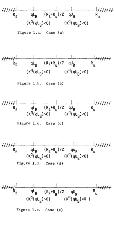
(Ru - R~) is at least halved after updating except the first iteration. Next, R is set to (R9., + R) /2 and same procedure is repeated. (Refer to Figure la Figure le in the proof of Theorem 2.)

[ Al

gorithm 1 ]

Step 0

Step 1

Step 2

Step 3:

Step 4:

Set R"" RI (n is an aribitrary positive numbert), R .... M(M is

1 tt u

a sufficiently large number ) and R9., .... 0. Go to Step 1. Solve P~ and find B, rB' tB' LB and VB. Go to Step 2.

If kq(qL_B) < 0, set Ru .... qL_B and R"" (R_u+R£)/2, and return to Step 1; if Jfl(qLB)=O, set S"" qL

B and go to Step 4; if Jfl(qL

B) > 0, go to Step 3.

If Jfl(qv_B) < 0, solve Q-equation and set S"" S2 or SI (according to LB;S S2;S VB or LB;S Sl,:s VB) and go to Step 4; i f Jfl(qvB)::o, set S .... qV B and go to Step 4; i f

KJ

(qV B) > 0, set R 9., .... qV Band R"" (Ru +R9.,) /2 and return to Step 1.

Set x(q).... : r_B + tB and terminate.

t If an optimal solution of certain subproblemp~ for q > q (or q < q) is

I " " I " "

known, then RI.;: x(q)'Vx(q) (Rl;S x(q)'Vx(q) ) should be taken as an RI·

-'

130 H. Ishii, T. Nishida and Y. Nanbu

Remark:

(1) Several methods to choose the next R are possible, and efficiency of Algorithm 1 seems to greatly depend on the choice method.

(2) If ~(qLB) < 0, ~(qUB) < 0 necessarily holds by Theorem 1. Thus the test for ~(qUB) is not needed. In case ~(qUB) > 0, ~CqLB) > 0 holds and the test for ~(qLB) is also omitted.

(3) [qLB'qU_B] ~ [R_Z' Ru] holds except the first L_B, UB'

Theorem 2.

Algorithm 1 terminates after finite iterations and it finds an optimal solution x(q) of pQ upon termination.

Proof: (Finiteness)

After each calculation of Step

1,

five cases Ca), Cb), Cc), (d), (e) ( as illustrated in Figure la, lb, lc, Id, and le below) are possible. (Note that the case of both ~(qLB) < 0 and ~(qUB) > 0 never occurs as pointed out in the above Remark.)

In case (d), (e), it is clear that

and

holds respectively. In case (c), either

SI

or

S2

(but not both) must belong to [qL

B, quB] according to the continuity and "the mean value theorem" with respect to ~ (R). In case (c), (d), (e), algorithm 1 jumps to Step 4 and terminates. In case (a), (b), neither

SI

nor

S2

belongs to the interval

~LB' qUE] by Theorem 1. First, note that (4.1) qL_B ~ (Ri +Ru )/2 ~ qUB

holds as is easily known from the updating procedure of R in Step 2 or Step 3. Case a Ru is set to qL_B as f/(qL_B) < O.

Case b R9. is set to qUB as RCqU

B) > O.

In any cases, it follows from (4.1) that the difference Ru - Ri is at least halved except the first execution of Step 2 and Step 3. Therefore, after finite iterations, case(c), case(d) or case(e) occurs since RCq) belongs to a certain interval [qL

B, qUB] with qUB- qLB >

O~

(Validity)

Termination condition itself proves validity of Algorithm

1.

0

t Even in the degenerate case, that is, LB=U

B, another base B exists such that ~ = U (or U- = L ) and U

B -

~ > 0 according to the theory of the pa¥amet¥ic

qua~rati~

programming. Therefore, without any loss of generality, qUB - qL

7rT; TJ

RQ,

qL B

(RQ,+Ru)/2

_{qU B}

(Kq( qL

_B

) <0)

(Kq( qu

_B

) <0)

Figure l.a. Case (a)

Figure l.b. Case (b)

I

J I I I J I I 71 J rrrJ

1//11/1

I

I

11 I I I J I I r, } (, rJ

qL B

(RQ,+R_u)/2

_{qU B}

Ru

(Kq(qLB»O)

(Kq(qUB)<O)

Figure l.c. Case (c)

f+lH+II----l---II----,I----+111I11I1

RQ,

_qLB

(RQ,+R_u)/2

_{qU B}

Ru

(Kq(qLB)=O)

(Kq(qUB)<O)

Figure l.d. Case (il)

132 H. lshii, T. Nishida and Y. Nanbu

'S. PrOr'erticsof pq . '.

In this se.cti'on, minimization ofg(x,(!) defined as (2.2) of Section 2 is discussed. g(x,q) is a convex function with respect to q > 0 for fixed x since

2

~u.L

dq2

for q > D. For each x E 5, h (x) is defined as follows: (5.1) h (x) ~ inf{g ex, q) Iq> O}

Then the optimal solution q ex) giving hex)

r - 2

.Jl

og ( A,

2rrx Vx (5.2)

o

by searching the zero point of

is given as follows:

, 1. 2

(x Vx<~)

I 2

(x Vx>

2fT )

because of convexity of g (x, q) with respect to q, where f (q) denotes the probability density function of the standard normal distribution N(O.I).

*

*

,

Theorem 3. The optimal solution (x , q ) of P , i f exists, satisfies

*

*

j

*,

*

Af lq ) , x (q ) Vx (q ) or q proof Proof is easy and so it is omitted. Since

*

>.. 2 log(----~*~I~--7*----q 2rrx Cq ) Vx (q ) < 1.2 log(---*~,~--~*-2rrx (q ) Vx Iq ) >..2 log ( : : : -2rrR 2. rn1n * * *

holds from this necessary condition of (x ,:q), i f q exists, an upper bound

*

of q (denoted by q ) can be given by

u 1.2 log (---::2.---2rrR . _m1n (5.3) q _u

=

2 '

where R min ~ min{x Vx

I

x E 5}

D (otherwise)

Here, we define a transformation T from r

=

{q > D} to r u { 0 }. 2' plays a princi'pal role in our algorithm given in the next section.

T:

I (x(q) Vx(a) < log( I 21TX (q) Vx(q) T(q)

o

(otherwise)

Note that T(q) is nondecreasing function of q because of property (iii)

*

*

*

*

and Theorem 3 states a necessary condition of q is q T(q), that is, q is a fixed point of T. Unfortunately, thi5 condition is not necessarily a sufficient condition.

Theorem 4.

for ql >

0

and q2

=

T(ql)'

*

q ~ [ql' q2] in case ql < q2 holds.

proof:

I f ql > q2' for any q € [q2' ql]'

T(q) - q < T(q) - q2 ~ T(ql) - 02

=

o.

holds (since T(q) is a nondecreasing function of q).

"

Therefore

q

does not satisfy the necessary condition of q ,

ql < q2' the proof may be similarly done.

In case

[]

Now, next property (vii) shows that I(B) is a continuous interval if not empty.

(5.4)

Property (vii) :

I(B)

=

~ or I(B) consists of a continuous interval.

proof:

Solving either inequality

1"Vt

-ID

B B < 2 q - 1'SV1'B or I 1'BVtB

+ID

2 I < q - 1'BV1'B

with respect to q~' , results Table I which shows property (vii)

t q

~j1'B ~1'B

cannot happen as is shown in Appendix 3 if q > 0 only considered.

134 H. Ishii, T. Nishida and Y. Nanbu

6. Algorithm for P

First some notations ar~ d~fined.

SN scanned region of q

t

qm g(qm) .~- min{g(q) Iq £ I(B)}

where - denotes ordinary "closure operation".

*

v current best value

'V 'V

(x, q) current best solution qc current searched q

optimal basis with respect to qc qM ~ min{q

I

q £ I(B

q )} for I(B ) ~ ~

c qc

*

The following algorithm 2 starts with q = q , tiN = (q , +00), V =+00,

'V '\0 C U U

x =~ and q=~. In Step 1, it solves pq using Algorithm 1 and find x(q ) and

a

the optimal basis B I(B) is then calculated by solving the inequality

q q

(5.4) and g(q) on I(~ ) is aetermined. Proceeding to Step 2, minimum point

t qc

q of g(q) is calculated. I f T(qm) q, g(q ) is compared with current best

m

*

*

'V 'V m m

*

value v and v , q, x is updated in Step 4 if v > g(q). While in case T(qm)

~

qm' i f _{SNUT(Bq )}

~

(0, +00), current (x(q) ,

q.v~)

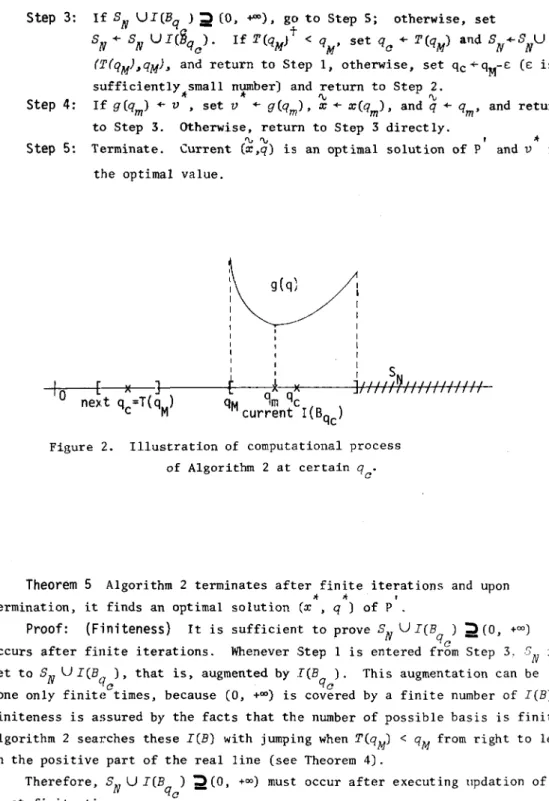
is optimal and

algorithm 2 terminates? Unless SNUI(Bq ) ~ (0, +00), SN is updated and augmented. Next qc is selected as follgws; if T(qM) < qw qc is set to T(qM): otherwise, qc is set to qM - £ where £ is sufficiently small positive number. Then, returing to Step 2 and above procedure is repeated. (see also Figure 2).

'r

tt

[ Algorithm 2 ]

*

'\0 'V

Step 0 Set qc+ qu' SN + (qu' +00), V + +00, X + ~ and q +~. Go to

Step

Step 2

Step 1.

Apply Algorithm 1 to problem pqc and calculate B_9c' x(qc) , I(B_qc) and determine g(q) on I(B_qc)' Go to Step 2.

Calculate q. _m I f T(q _m

)tt=

q , go to Step 4; _m otherwise, go to Step 3.

If qm is not unique, then we take the smallest one among these qm' Even i f q

i

I(B_{q ),} T(q ) can be calculated by continuity of T(q) as

m c m

1im T(q) and continuity of T(q) is assured by the continuity of x(q). q+qm+O

Step 3: I f SN UI(B_{q )} ~ (0, +",,), g~ to Step 5; otherwise, set SN +- SN U I (Bqc) . I f T(qMJ < qM' set qc +- T(qM) and SN+-SNU

(T(qMJ.qMJ. and return to Step 1, otherwise, set qc +-qM-e: (e: is sufficiently small number) and return to Step 2.

" " IV IV

If g(qm) +- v , set v +- g(q_), x+- x(q ), and q +- q , and return

"I m m

Step 4:

to Step 3. Otherwise, return to Step 3 directly.

Step 5: Terminate. Current (x,q) '\, '\, is an optimal solution of P and I v " is the optimal value.

l i S

I

E ] .L ~ /1 11 IN I J I ( I J I I I I /

-+O~--4---~x---~---+---~x~*X---]HJ~J~J+J+J+f+rJ+J+JhJhJ~J~J~J~J+J-next qc =T( qM) qM

9

m qc

current I(B_qc)

Figure 2. Illustration of computational process of Algorithm 2 at certain qc'

Theorem 5 Algorithm 2 terminates after finite iterations and upon

" "

,

termination, it finds an optimal solution (x , q ) of P .

Proof: (F-initeness) I t is sufficient to prove SN U I(B

q ) ~ (0, +00)

. C

occurs after finite iterations. Whenever Step 1 IS entered from Step 3. 5 N is set to SN U I(B l ), that is, augmented by _r(B ). This augmentation can be

'c ~

done only finite times, because (0, +00) is covered by a finite number of I(E). Finiteness is assured by the facts that the number of possible basis is finite. Algorithm 2 searches these I(E) with jumping when T(qM) < qM from right to left on the positive part of the real line (see Theorem 4).

Therefore, SN UI(E )

':leo,

+00) must occur after executing llpdation of qc

136 H. Ishii, T. Nishida and Y. Nanbu

(Validity)

Algorithm 2 scans (0, +00) and finds all q on I(B) except skipped

" m

interval (T(qM),qM] with assurance that q does not exist in the latter

"

Moreover, it is clear by Theorem 3 that optimal q interval by Theorem 4.

exists among such qm if exists. Therefore, upon termination, algorithm 2 has scanned all possible qm' This proves validity of Algorithm 2.

0

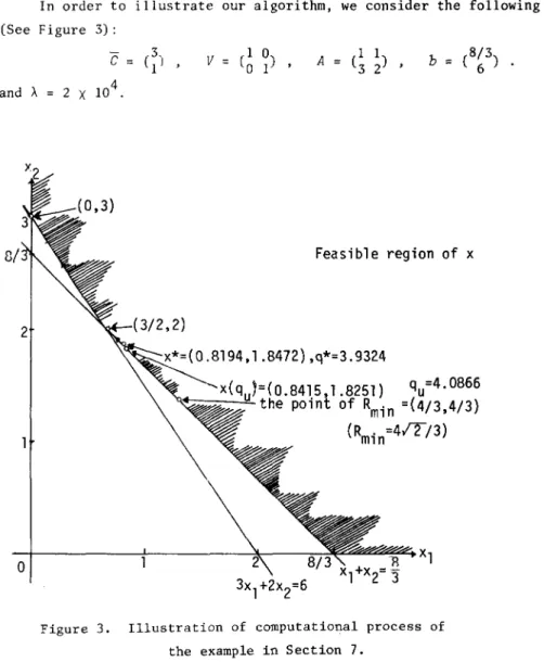
7. Example

In order to illustrate our algorithm, we consider the following example. (See Figure 3): and A

o

Figure 3.

c

=

(3. 1 '

v

A b

Feasible region of x

(0.8194,l.8472),q*=3.9324

'=(0.8415,1.8251)

qu=4.0866

"<\..+;=:-:--~

_{the point of Rmin =(4/3,4/3)}

(R

min

=4/"2/3)

Illustration of computational process of the example in Section 7.

I

Then P becomes as follows:

t P

Step 0

Step 1

I minimi ze 3x l + x2 +

J1---;-;Z -

. I 2 20000 F (q) subject to xl + x 2 ~ 8/3 qc ~ quC= 4.0866). Go to Step l.

(Algorithm l)t

3x l + 2x2 ~ 6 Xl,x2~O. q>O.

Step 0

Step 1

Set R ~ RI (=2q ),R ~ M u u and Ri ~ O. u l xl x2 el B

[1

-1 0

-~]

0 -1 =(6/13 ) 1 1 1'B 9/13 1'B 3 2 14/9 . U _B 3 Go to Step 2. Go to Step 1. =

C

8 / 13 ) 12/13 LB

Step 2

Since

JfI

(q cLB) < 0, _{set Ru} +- qcLB(=qu

14

x - - ) and

9

R~ (R _u + R_i)/2(=7/9 q ), _u and return to Step 1. u 1 u2 xl x2 1'B =c) 2/3 1'B 2

[1

3 -1

J

2 0 B 0 1 0 3 LB 2/3 liB 14/9 Go to Step 2.

138

Therefore,

Step 2

Step 4

Step 3

H. Ishii, T. Nishida and Y. Nanbu

Go to Step 2.

Step 2

Step 1

B =

Step 2

Step 3

](1 (qcLB) < 0, R + q L B(=2/3 q ) u e u R + 1/3 q . _u Return to Step 1. u l xl x2 e2 =

(~)

e/

3 ) r B tB = 4/3

[f

-1 0

-~]

0 -1 1 1 L = _B

o ,

U_B = 2/3 • 3 2 Go to Step 2. Since ~(qcLB)

=

4~/3 > 0, Go to Step 3. Since ~(q _UB) = 2~/3 - 2/3 q < 0, c , , u , solve

Q

equation (rBVtB= 0 _rBVrB = 2 tBvt_B = 9/32) {(q )2 _ 2}R2 _ 32/9 q2 = 0 u e and set ~ +

6

2 (=0.4918 q ) because of 2 ' 2 u qc - rBVrB

=

qu - 2 > O. Go to Step 4.

Step 4

Terminate. 0.8415

li

x(qc) _{= 1. 8251} B qc r B qc (-1, 1) , _{tB' = (4/3, 4/3), LB} 0, qc qc I(Bq )

=

[_~ +00) C ';'-=2--and g(q)

=

(4~ /3)' q - 2 Go to Step 2. q = 3.9324 m

*

qM =~. Since T(q ) m

=

q , m Since v (="")

*

> g(q ) _m = -19992 '2811, set v + g(q )(= -19992.2811), -1 0 1 3 U B qc 0

-~]

-1 1 2

=

2/3 - 20000 F(q). Go to Step 4. '" _{x + x(q} m _{)(= (0,8194,} m

,

'"

1.8472) ) and q + q (=.3.9324), m Return to Step 3.

Since SNLJI(Bqc) ~ [~, +00) C:(O, +00) set SN + SN U I(Bqc ) (=t.Ii'i)", +00))

As T(qM) = 3.884726 > qM =

liD

= 3.162277, set q + qM - E: and

return to Step 1.

Since the serial computational routines are almost same as above, results only are enumerated.

q =110- £ c LB qc 3 2

o

o 2/3 Xl -1 0 3 x 2

-lB

_q(J

·G)

2 U B = 14/9 . qc

{2~3

), t8 qc qM 3110/7 < T(qM) 3.884726 and SN ... [3110 /7, +00) • qc 3110/7 - £ u l X 1 x2 e1

[;

-1 0 -1 0

_-IJ

_=(6/13 ₎ =(8/1 3 ) B = 1"B tB qc 1 _q 9/13 _q 12/13 3 2 LB 14/9 U B _{3 .} qc qc I(Bq ) = [1, c 3110 /7], qM = 3110 /7 # T(qm) , T(qM) > qM = 1. and SN ... [1, +00) • qc = 1 - £ : _{vI u} 2 x2 el _1"B =G) tB =G) qc qc

~

3 0

-~]

2 -1 LB U_B B = ₀ 3. +"". qc 1 qc qc 0 2

;(Bqc)

=

(0, 1], qM =,qm

=

0* and _{SN UI(Bqc)} ~(O, +00). Terminate X = ( 0.8194, 1.8472) and q = 3.9324.

8. Concl usion

The most difficult point in our algorithm is to find qm in Step 2. Since g(q) is a function of q only, we may manage to obtain qm if the form of g(q) on I(B ) is known. The second difficult point is a lack of sufficient condition

q

*

about q. Especially in this problem, the lack of useful suffiCient condition urges us to search all possible points with T(q)=q, among all positive q.

Note that for fixed a, our problem is equivalent to Kataoka's problem [6]. But even in such case, our method may be considered as a different approach.

140 H. Ishii. T. Nishida and Y. Nanbu

Although the effect of rx on thE' objective function was taken as -Aa, there may be othE'r ways to includE' thE' effE'ct of a. In such cases, however, the problem may become more complicated and more difficult to solvE'. Admitting the linearity of the effect of a, in practical situation, the domain of a may be more restricted.

9. Acknowledgement

The authors would like to thank Professor H. Mine and Associate Professor T. Ibaraki of Kyoto University for their valuable comments and suggestions, and are greatly indebted to S. Shiode of Osaka University for completing this paper.

References

[1] Charnes, A. and Cooper, W.W. : Chance Constrained Programming. Management Science Vo1.6 (1959)., pp73-79.

[2] Charnes, A. and Cooper, W.W. Deterministic Equivalents for Optimizing and Satisficing under Chance Constraints. Operations Research vol.ll (1963), pp18-39.

[3] Charnes, A. and Kirby, M.J.L. : Some Special P-models in Chance Constrained Programming. Management Science Vol.14 (1967), pp183-195.

[4] Eism~r, M.J., Kaplan, R.S. and Soden, J.V. : Admissible Decision Rules for the E-Model of Chance-Constrained Programming. Management Science Vol.17 (1971), pp337-353.

[5] Gor-het, W.F. and Padberg, M.V. : The Trianglu1ar E-Model of Chance-Constrained Programming. Operations Research Vol.19 (1971), pp105-114. [6] Kataoka, S. : A Stochastic Programming Model. Econometrica Vo1.31 (1963),

pp18l-l96.

[7] Kirby, M.J.L. : The current State of Chance-Constrained Programming. Proceedings of the Princeton Symposium on MathematicaZ Programming (Ed. H. W. Kuhn) Princeton University Press, Princeton, New Jersey, 1970, pp93-ll1. [8] Mangasarian, O.L. : NonZinear Programming Mcgraw-Hill, 1969.

[9] Sengupta, J.K. : Stoehastic Programming North Holland, Amsterdam, 1972. [10] Vajda, S. ProbabiUstic Programming Academic Press, 1972.

[11] Wo1fe, P. The Simplex Methods for Quadratic Programming. Econometrica Vol.27 (1959), pp382-398.

IIiroaki Ishii and Toshio Nishida:

Department of Applied Physics, Faculty of Engineering, Osaka University, Yamada-kami, Suita, Osaka, 565, Japan.

Appendix

Derivation of

pI

The chance constraint in (2.1) can be transformed into the following form by simplex subtrction and devision.

, -, j' -, (A-I) Pr>cb( c'x<.:.fJ = Prob(e x-a

Xs:

-a x

- 1:::'Vx -/x'Vx

Since a is distributed according to N(~, VJ, a'x - ~'x

1X'Vx-can be considered as a normalized random variable with zero mean and unit vari-ance (that is, standard normal distribution). Therefore (A-I) is replaced by

f~~'x + P-l(a.Jlx'Vx

where P is the distribution function of standard normal distribution, N( 0,1 J. Since minimum of f is attained when the equality holds. setting

-1

q

=

P (a.),

the objective function becomes as follows c'x + qlx'Vx -AP(qJ.

Appendix 2 Proofs of Properties (i) - (iv)

(i) It is clear from the strict convexity of the objective function and the fact that S is convex set.

( i i) For q 2 > -11 >

° ,

c'x(Q2) + q ix (q2) 'Vx(q2) >c'x(q~:) +q/x(q2) 'V:::(q2) ( q2 >ql)

~ ~'x(ql)

+q/x(ql) 'Vx(ql) (optimality of q1 for pql).

(iii)

For q2 >q1 > 0, from the optimality of x(ql)' x(Q2) , (A-2) ~'x(ql) +q/x(ql) 'Vx(ql) ~~'x(q2) +q

l/x(q2) 'Vx(q2) (A-3) ~ 'x(q;:;) +q i x ( q 2) 'Vx( q 2} ; ;; 'x(qlJ +q/x( ql} 'Vx( ql}

142 H. lshii, T. Nishida and Y. Nanbu

holds. The assumption (q2- q l) > 0 implies v'x(ql} 'Vx(ql} ~ v'x7q 2} 'Vx(q2}' (iv) From Property (iii),

(A-S) c'x(ql) +q/x(q]} 'vx(ql} ~c'x(Q2) +q

lv'x(q2} 'Vx(q2} ;c'x(q2) +q/x(ql} 'Vx(QI}

holds. (A-S) implies c 'x(q ) < c 'x(q ) I

=

2

Appendix 3

q~v'piVPB Assume q=v'rBVP B £BVtB R(q)

=

2r

B

VtB holds. Since

for an optimal basis B

R() _tBVtB

Then~=

2 'Vt

q P_B B from Q equation, that is,

R(g) . .0 x(q) = P +t B and K'(R(q)) =0, q B 2 R2 R( ) 2 x(q) 'Vx(q) -R(q)

=7

P_BVP_B+ 2 - T PBVtB+tBVtB-R(q) P BVPB(tBVtB) 2 , , PBVPB(tBVtB) 2 4 (PBVt B) 2 - + tBVtB + tBVtB 4 (PBVtB) 2 2t

BVtB=O, or t;B=O. (For V is positive definite matrix.) This implies

..!i.fsJ.l

=0 ' or R(q) =x(q) 'Vx(q)

=

0, or x(q)=O.

Q

Since again V is positive definite matrix,

x(q)=O and tB=O together implies PB=O or q=O. We considers only q > 0 and so q = v'P;VP B cannot happen.

Appendix 4 Kuhn-Tucker condition of Problem

P~

for the example.

- R

v + A 'u - Vx = ( J '

-q

Ax-e=b, u'e+v'x=O, u, v, eJ x~O, that is,

R VI +u_I +3u₂ -xl

=

3-q R v 2+uI +2u2-x2

=-q

D

o

x +X -e =8/3 1 2 1

3x I + 2x 2 - e 2

=

6

xlVI +x_{2v 2+e l}u_{l +e2u 2 =o,} xl' x'2' vI' v

2' el' e2, uI' u 2 ;O.

Appendix 5.

Table 1. I (B) •

Case Subcase I(B)

rsVtB ~ 0 {q\A₂;q;A,}

A4~A5 & A4 > 0 {q

I

q>Aa & A2~ q ~A, } A7 < 0, A5 > 0 & A5;A4 {q

I

_{q<Aa & A2; q ;A,}}

I,

A7 ~ 0, A6 < 0, A5 < 0 & {q

I

q<A8 & A₂; q ;A, } A3 ; A2 ; A,

A7 ~ 0, A6 < 0 & {q

I

q<Aa & A, ~ q ~Ag} A2 ; min (A, ,A₃)

rsVtB < 0 A7 '? 0, A6 < 0 & _{qlq<A8 & min(A2,A3)~q~Ag} }

A, ~ min (A₂,A 3) A6 ~ 0, A4 < 0, A3~A2 & A, ; min (A₂

NA6 )

{qlq<A_a & A2~q~A,}

A6 f: 0 & maxVA;5,A₂) _{q

_I

_{q<Aa & Ag~ q ~A, }} A4<0, A6~0, A3,;A2 & _{qlq<Aa & A,,; q ,;A3}

Al;~

A6 ~ 0 & {qlq<A_a & Ag;:i q ;:imin(A 2,A3)}

VAi

;:iA,;:i min(A₂,A₃)

144 H. Ishii, T. Nishida and Y. Nanbu

In Table 1,

Note that