k519 fulltext

(1)

Pattern recognition based on naive canonical correlations

in high dimension low sample size

March, 2014

Mitsuru Tamatani

(2)

Abstract

This paper is concerned with pattern recognition for K(≥ 2)-class problems in a High Dimension Low Sample Size (hdlss) context. The proposed method is based on canonical correlations between the predictors and response vector of class label. This paper proposes a modiﬁed version of the canonical correlation matrix which is suitable for discrimination of a new data in a hdlss context. We call such a matrix the naive canonical correlation matrix which plays an important role in this paper. Provided the dimension does not grow too fast, we show that the K− 1 sample eigenvectors of naive canonical correlation matrix are consistent estimators of the corresponding population parameters as both the dimension and sample size grow, and we give upper bounds for the misclassiﬁcation rate. Furthermore, we propose variable ranking and feature selection methods which integrate information from all K − 1 eigenvectors. For real and simulated data we illustrate the performance of the new method which results in lower errors and typically smaller numbers of selected variables than existing methods.

(3)

1 Introduction

Pattern recognition is a statistical method by which a new data with unknown class label is classiﬁed into one of the previously known classes. Generally, the overall process can be divided into four main steps: preprocessing of data, feature extraction, feature selection, and discrimination. Following Devroye et al. (1996), we use the notion Pattern Recognition synonymously with Discrimination, and consider the problem of classifying d-dimensional random vectors X into one of K classes.

Fisher’s well-known linear discriminant function for K-class problems is the solution to his paradigm: maximize the between-class variance while minimizing the within-class variances. See Fisher (1936), and Rao (1948) for the general multi-class setting. Especially, for the special case of 2-class problems, we assume that the two populations, C1 and

C2, have multivariate normal distributions which diﬀer in their means µ1 and µ2, but

share a common covariance matrix Σ. For X from one of the two classes, Fisher’s linear discriminant function g(X) = ( X− 1 2(µ1+ µ2) )T Σ−1(µ₁− µ₂) (1.1)

assigns X to C1 if g(X) > 0, and to C2 otherwise. If the random vectors have equal

probability of belonging to either of the two classes, then the misclassiﬁcation rate of (1.1) is shown to be 1 2 [ Φ ( −∆2 2 ) + { 1− Φ ( ∆2 2 )}] ,

where Φ is the standard normal distribution function and ∆ is the Mahalanobis distance between the two populations:

∆ = √ (µ₁− µ₂)TΣ−1(µ₁− µ₂). A sample version of (1.1) is bg(X) = ( X−1 2(bµ1+bµ2) )T bΣ−1₍_bµ 1− bµ2), (1.2)

wherebµ₁,bµ₂and bΣ are appropriate estimates for the corresponding population parameters of the two classes. (1.2) can be applied to data sets in the general setting where the

(6)

sample size n is much larger than the dimension d. However, for problems with a large dimension, it has been shown that Fisher’s linear discriminant function performs poorly due to diverging spectra. Further for High Dimension Low Sample Size (hdlss) problems, namely n ≪ d, it is not possible to directly deﬁne Fisher’s linear discriminant function since the sample covariance matrix bΣ in (1.2) becomes singular when the dimension d exceeds the sample size n.

Several discriminant rules have been proposed for the hdlss context which overcome the problem of singularity of bΣ in diﬀerent ways: Dudoit et al. (2002) proposed diagonal linear discriminant analysis which only uses the diagonal elements of the sample covariance matrix, Srivastava and Kubokawa (2007) proposed a discriminant function based on the Moore-Penrose inverse, Ahn and Marron (2010) constructed discriminant function based on the Maximal Data Piling (MDP) direction vectors, and Aoshima and Yata (2011) considered a discriminant rule based on second moments in conjunction with geometric representations of high-dimensional data.

In this paper we focus on the ‘diagonal’ approach of Dudoit et al. (2002) which has special appeal since it is conceptually simpler than the competitors. Further, this approach can be implemented eﬃciently for large and complex data sets. We refer to Fisher’s linear discriminant function based on the diagonal of the covariance matrix as the naive Bayes rule.

For two-class problems in a hdlss setting, Bickel and Levina (2004) and Fan and Fan (2008) investigated the asymptotic behavior of the naive Bayes rule, and calculated bounds for its misclassification rate. Tamatani et al. (2012) defined a modification of the canonical correlation matrix that is suitable for classification problems, and studied the asymptotic behavior of the eigenvector and the discriminant direction of the modified canonical correlation matrix in the context of two-class problems. Also, for multi-class problems in a hdlss context, Tamatani et al. (2013) proposed a naive Bayes rule in a general multi-class setting and investigated its asymptotic properties for high-dimensional data when both the dimension d and the sample size n grow.

(7)

Throughout this paper we focus on hdlss data from K(≥ 2) classes, that is, we assume that the dimension d of the data is much bigger than the sample size n. Our discriminant approach is based on canonical correlations, and in particular on a modification of the canonical correlation matrix suitable for vector-valued class labels from K classes. In this framework, we replace the covariance matrix by its diagonal counterpart as discussed in Dudoit et al. (2002), Bickel and Levina (2004) and Fan and Fan (2008). We call such a matrix the naive canonical correlation matrix, and observe that this matrix plays an important role in the present theory. The K − 1 eigenvectors belonging to K − 1 non-zero eigenvalues of the estimated naive canonical correlation matrix yield discriminant directions which inform our choice of a discriminant function for K classes. For this setting we study the asymptotic behavior of the eigenvectors and associate discriminant directions. In principal component analysis, Johnstone (2001) proposes the notion of spiked covariance matrices and Ahn et al. (2007) and Jung and Marron (2009) combine the spikiness of the covariance matrix with hdlss consistency. hdlss consistency is a measure of the closeness of two vectors in a hdlss setting, and is given in terms of the angle between the vectors. Ahn et al. (2007) and Jung and Marron (2009) derive precise conditions under which the first eigenvector of the sample covariance matrix is hdlss consistent. These conditions include the asymptotic rate of growth of the first eigenvalue which exceeds the dimension d. Like Ahn et al. (2007) and Jung and Marron (2009), we consider the asymptotic behavior of K− 1 eigenvectors in a hdlss classification context. In our context, however, their spiked covariance model is not appropriate since we are dealing with inverses of the covariance matrix. As a result, our conditions for consistency differ considerably from theirs.

For hdlss data from K multivariate normal classes, we derive an upper bound for the misclassiﬁcation rate of the proposed multi-class discriminant function. Our asymptotic results for the misclassiﬁcation rate are divided into two disjoint types depending on the precise growth rates of d and n. Depending on the two distinct growth rates, we also develop hdlss asymptotic results for estimators of the eigenvectors and discriminant

(8)

directions.

In high-dimensional settings, it is necessary to select a subset of relevant features (or variables) for discrimination. There are several discussions on feature selection methods for multi-class discriminant analysis, see Saeys et al. (2007). It appears that many of these proposals are variable selection methods which are not speciﬁc for or connected with a par-ticular discriminant function. We believe that in discriminant analysis, a comprehensive feature selection method should include the discriminant function in the variable ranking and in the choice of the number of selected features. We propose new feature selection methods speciﬁcally for our multi-class discriminant function.

The paper is organized as follows. In Section 2, we review the framework of pattern recognition and a relationship between Fisher’s rule and canonical correlations for K classes. This relationship explicitly exhibits Fisher’s ratio of the within-class and between-class variances, and its maximizer provides a discriminant rule. In Section 3, we focus on the gene expression microarray data, which is a typical example of hdlss data. In general, hdlss data are emerging in various areas of modern science such as genetic microarrays, medical imaging, text recognition, chemometrics, face recognition, and so on. Further, we present a similar discussion in Section 2 for hdlss data; we replace Σ by diagΣ, and obtain a corresponding criterion, which leads to a natural derivation of a multi-class version of the naive Bayes rule. Section 4 details the asymptotic behavior of the eigenvectors of the estimated naive canonical correlation matrix and the associated discriminant directions in a hdlss setting under general distributional assumptions. We derive an upper bound for the asymptotic misclassification rate of the proposed multi-class discriminant function under assumptions of normal distribution, and we show that the upper bound for the asymptotic misclassification rate is indeed a multi-class extension of that obtained in Fan and Fan (2008) and Tamatani et al. (2012). Section 5 includes new feature selection methods for K-class discriminant analysis, which naturally follow from our analysis of the naive canonical correlation matrix. Section 6 provides numerical studies to validate the theorems derived in Section 4. Our numerical results confirm the asymptotic behavior of

(9)

discriminant directions of Subsection 4.3, and an upper bound for the misclassiﬁcation rate of the multi-class discriminant function proposed in Subsection 4.4. Furthermore, we apply proposed methods in Section 5 to simulated data sets, and compare the performance of our methods with other ranking methods. Section 7 applies the proposed methods in Section 5 to microarray data example and English spoken data. These comparisons demonstrate that our feature selection methods work well and yield a parsimonious set of features which lead to good classiﬁcation results. Section 8 contains proofs of our theoretical results. In Section 9, we summarize our results and survey related works and directions for future research.

(10)

2 Pattern Recognition

2.1 Problem of Pattern Recognition

Let K be the number of class labels. For observation vector x∈ Rd belonging to a class k∈ {1, . . . , K}, we deﬁne the function g, which is called discriminant function, as

g :Rd −→ {1, . . . , K}.

For evaluating the accuracy of the discriminant function g, it is important to focus on the probability

P (g(X)̸= Y ),

which is called misclassiﬁcation rate of g, where X is a new data taking value in Rd _and Y is the class label of X taking value in{1, . . . , K}. Our purpose is to choose a function g∗ such as misclassiﬁcation rate is small, that is, for any discriminant function g,

P (g∗(X)̸= Y ) ≤ P (g(X) ̸= Y ). (2.1)

(2.1) means that g∗ is the optimal function, which is called the Bayes rule (see Devroye et al. (1996)).

In the following sections, we ﬁrst consider two-class problem under normal distributions and then investigate the extension to general multi-class discriminant problems. The aim of these sections is to relate Fisher’s linear discriminant function and canonical correlation analysis.

2.2 Fisher’s Linear Discriminant Function

In this subsection, we consider two-class setting. Let C1 and C2 be two d-dimensional

populations with diﬀerent means µ₁ and µ₂ and the same covariance matrix Σ. For a

random vector X from one of these populations/classes, let π1 be the probability that X

(11)

Linear discriminant function is obtained by projecting observation vector x to one dimension using

z(a) = aTx, (2.2)

where a is called a weight vector. For x from one of the two classes, (2.2) assigns x to C1 if z(a) ≥ −a0, and otherwise class C2, where a0 is a threshold. A characteristic of

(2.2) is that it is easier to interpret than nonlinear functions. In addition, we can select a projection that maximizes the class separation by adjusting the components of weight vector. Here an important point is that we need to ﬁnd an eﬃcient weight vector which maximizes the separation between classes.

Fisher’s idea is to obtain the vector a which maximizes the ratio of the between-class variance ΣB and within-class variance ΣW:

J∗(a) = a T_Σ Ba aT_Σ Wa , (2.3) where ΣB = (E[ X | C1 ]− E[ X | C2 ]) (E[ X | C1 ]− E[ X | C2 ])T = (µ₁− µ₂)(µ₁− µ₂)T and ΣW = 2 ∑ ℓ=1 πℓV [ X | Cℓ ] = 2 ∑ ℓ=1 πℓE[ (X− µℓ)(X− µℓ)T | Cℓ ] = Σ.

As is well known, a solution of a∗ _{= arg maxa}_∈Rd_−{₀_}J∗(a) is given by

(12)

see e.g. Bishop and Nasrabadi (2006). Here we select the value a0(a∗) = 1 2(E[ Z(a ∗₎ _{| C} 1 ] + E[ Z(a∗) | C2 ]) = 1 2a ∗T_(µ 1+ µ2)

as the threshold using (2.4). Therefore, the linear discriminant function g∗(x) = z(a∗)− a0(a∗)

becomes (1.1), and is called Fisher’s linear discriminant function or Fisher’s rule. It is also well known that the choice (2.4) yields the Bayes rule, see Devroye et al. (1996).

2.3 Discriminant Function Based on Canonical Correlations

In this subsection we review the relationship between canonical correlations and Fisher’s linear discriminant function in pattern recognition.

In canonical correlation analysis of two subsets of variables X[1] and X[2] of a random

vector X = [ X[1] X[2] ] , (2.5)

the canonical correlation matrix

C_∗ = Σ−1/2₁ Σ1,2Σ−1/22 , (2.6)

and the derived matrix C_∗C_∗T play important roles, see Mardia et al. (1979). Here Σℓ is

the covariance matrix of X[ℓ] (ℓ = 1, 2), and Σ1,2 is the between-covariance matrix of the

two vectors: Σℓ = E [ (X[ℓ]− E[X[ℓ]])(X[ℓ]− E[X[ℓ]])T ] , Σ1,2 = E [ (X[1]− E[X[1]])(X[2]− E[X[2]])T ] .

For random vectors X belonging to one of the classes C1 and C2, we replace X[1] in

(2.5) by X, and X[2] by the vector of labels Y deﬁned by

Y = [ Y1 Y2 ] and P (Y = eℓ) = πℓ, (2.7)

(13)

where eℓ is the vector with ℓth entry 1 and 0 otherwise. For X and Y we deﬁne the

matrix

e

C = Σ−1/2E[(X− µ) YT] {E[Y YT]}−1/2, (2.8) where µ = π1µ1+ π2µ2. Strictly speaking, the centered Y should be used for eC in (2.8),

however, for the vector of labels Y , centering is not meaningful. From (2.7) and (2.8) it follows that E[Y YT] = [ π1 0 0 π2 ] , E[(X− µ) YT] = E[XYT]− µE[YT] = [ π1µ1 π2µ2 ]− µ[π1, π2] = [ π1(µ1− µ) π2(µ2− µ) ], and hence e C eCT = Σ−1/2M Σ−1/2, (2.9) where M = E[(X− µ) YT] {E[Y YT]}−1E[(X− µ) YT]T = 2 ∑ ℓ=1 πℓ(µℓ− µ)(µℓ− µ)T.

Now, consider the eigenvalue problem eC eCTep = ˜λep. Using the expression (2.9), we see that solving the eigenvalue problem is equivalent to maximizing eJ (b) deﬁned by

e J (b) = b T_{M b} bTΣb. (2.10) From M = 2 ∑ ℓ=1 πℓ(µℓ− µ)(µℓ− µ)T = π1π2(µ1− µ2)(µ1− µ2)T = π1π2ΣB,

(14)

2.4 Fisher’s Rule for Multi-class

We consider the K-class discrimination problem. Let Cℓ (ℓ = 1, . . . , K) be d-dimensional

populations with diﬀerent means µ_ℓ and common covariance matrix Σ. For a random vector X from one of the K classes, let πℓ be the probability that X belongs to Cℓ. Let

Y be the K-dimensional vector-valued class label with ℓth entry 1 if X belongs toCℓ and

0 otherwise, so P (Y = eℓ) = πℓ, and

∑K

ℓ=1πℓ = 1.

In canonical correlation analysis of two vectors X and Y , with Y the vector-valued labels and µ =∑K_ℓ=1πℓµℓ, the matrix (2.8) plays an important role. From the deﬁnition

of (X, Y ) it follows that

E[Y YT] = Π and E[(X− µ)YT]= M0Π, (2.11)

where Π = diag(π1, . . . , πK) and M0 = [ µ1− µ · · · µK− µ ]. Using

M =

K

∑

ℓ=1

πℓ(µℓ− µ)(µℓ− µ)T = M0ΠM0T,

we have (2.9). If we put eb = Σ−1/2ep, where ep is a solution to the eigenvalue problem e

C eCTep = ˜λep with ˜λ > 0, then the vector eb is the maximizer of the criterion e

J (b) = b T_{M b}

bTΣb (2.12)

over vectors b. Note that (2.12) is nothing other than the criterion which yields Fisher’s rule for the multi-class setting. In particular, the rank of eC eCT is K − 1, so the K − 1 eigenvectors [ ep₁ · · · ep_K₋₁ ] belonging to K− 1 non-zero eigenvalues should be used for constructing the discriminant directions

e

B ≡ [ eb1 · · · ebK−1 ] = Σ−1/2[ep1 · · · epK−1 ].

Using the discriminant directions eB, we want to deﬁne a discriminant function eg for classifying new observations X whose class is unknown. For α ∈ {1, . . . , K − 1}, put Zα(X) = eb

T

αX, and deﬁne the vector Z(X) = [Z1(X), . . . , ZK−1(X)]T = eBTX. For

Z(X) andCℓ, deﬁne the Mahalanobis distance between Z(X) andCℓ by

∆ℓ(Z(X)) =

√

(15)

where

νℓ= E [ Z(X)| Cℓ ] = E [ Z(X)| Y = eℓ ] = eBTµℓ

and

Σℓ= V [ Z(X) | Cℓ ] = V [ Z(X) | Y = eℓ ] = eBTΣ eB.

Hence ∆ℓ(Z(X))2 can be rewritten as

∆ℓ(Z(X))2 = (X− µℓ) T e

B( eBTΣ eB)−1BeT(X− µ_ℓ) . (2.13) Using (2.13), we now derive the multi-class discriminant function eg as the minimizer of the Mahalanobis distance, and let

eg(X) = arg min

ℓ∈{1,...,K}

∆ℓ(Z(X))2. (2.14)

Note that eB depends on Σ and that (2.14) reduces to the Fisher’s linear discriminant function in the case of 2-class by considering the sign of ∆1(Z(X))2− ∆2(Z(X))2.

2.5 Other Discriminant Functions

In previous subsections, we introduced Fisher’s rule and discriminant function based on canonical correlations. Another discriminant functions have been discussed in literatures which include empirical risk minimization method, nearest neighbor rule, kernel method, neural network, and so on (see Devroye et al. (1996), Bishop and Nasrabadi (2006), Duda et al. (2012)).

3 HDLSS

3.1 HDLSS Setting

Gene expression microarray data is a form of high-throughput biological data providing relative measurements of mRNA levels for genes in a biological sample. One important application of gene expression microarray data is the classiﬁcation of new samples into

(16)

known classes. In the recent years, many laboratories have collected and analyzed mi-croarray data, and such data have been appeared in public databases or on web sites. Indeed, the data collected from gene expression microarrays consist of thousands or tens of thousands of genes that constitute features: leukemia data (Golub et al. (1999), K = 2, n = 73, d = 7129), lung cancer data (Gordon et al. (2002), K = 2, n = 184, d = 12433), prostate cancer data (Singh et al. (2002), K = 2, n = 134, d = 12600), the small round blue cell tumors (SRBCT) data (Khan et al. (2001), K = 4, n = 83, d = 2308), and so on. These data, often called the High Dimension Low Sample Size (hdlss) data, are characterized with large number of dimensions d and a relatively small number of sample size n, that is, we can write n≪ d.

To establish asymptotic theory in this paper, we consider an asymptotic situation in which the dimension d and the sample size n both approach inﬁnity in such a way that d is much faster than n:

n = o(d) as n, d −→ ∞.

3.2 Diﬃculties in HDLSS

The hdlss data involves serious problems. Let Xi (i = 1, . . . , n) be independently and identically distributed (i.i.d.) d-dimensional random vectors with the covariance matrix Σ. The usual estimates of Σ is deﬁned as

bΣ = 1 n− 1 n ∑ i=1 (Xi− bµ)(Xi− bµ)T, (3.1)

where bµ = (1/n)∑n_i=1Xi is the mean vector of the data {Xi}1≤i≤n. When we assume

that the data satisﬁes n ≪ d, (3.1) is a singular matrix because the rank of (3.1) is at most n− 1. Hence, it means that the sample version of (2.8) is not directly applicable in the case of n≪ d.

The difficulty of high-dimensional classification in data analysis is intrinsically caused by the existence of many noise features that do not contribute to the decrease of misclas-sification rate. To avoid the above problem, the importance of feature selection has been

(17)

stressed and several methods of feature selection for hdlss data have been proposed in literatures, for example, nearest shrunken centroids method (Tibshirani et al. (2002)) , fea-ture annealed independence rules (Fan and Fan (2008)), minimum redundancy maximum relevance feature selection (Ding and Peng (2005), Peng et al. (2005)), and so on.

3.3 Naive Canonical Correlations

In the hdlss two-class discrimination settings, the sample covariance matrix bΣ is singular as was discussed in the previous subsection. For a population framework, it therefore does not make sense to define a discriminant function based on the within-class covariance matrix Σ. To overcome such a difficulty, we first require a suitable framework for the population. We define the naive canonical correlation matrix C and vectors bα and pα by

C = D−1/2E[(X− µ)YT] {E[Y YT]}−1/2

and bα = D−1/2pα, where D = diagΣ, and pα is eigenvector of the matrix CCT

corre-sponding to the αth largest eigenvalue λ∗_α. Put P = [ p₁ · · · p_K₋₁ ]. The discriminant directions

B ≡ [ b1 · · · bK−1 ] = [ D−1/2p1 · · · D−1/2pK−1 ] = D−1/2P

can now be seen to maximise the analogous naive criterion J (b) = b

T_{M b}

bTDb. (3.2)

Note that Σ in (2.12) has been replaced by the diagonal matrix D in (3.2).

3.4 Discriminant Function in HDLSS

The corresponding discriminant function g is therefore g(X) = arg min

ℓ∈{1,...,K}

(X− µ_ℓ)TB(BTDB)−1BT (X− µ_ℓ) . (3.3)

Note that Σ has been replaced by D both in (2.12) and (2.13) to yield (3.2) and (3.3) respectively.

(18)

It is worth noting that for K = 2, the discriminant function g reduces to the naive Bayes discriminant function discussed in Bickel and Levina (2004).

4 Asymptotic Theory

In this section, we evaluate the asymptotic behavior of the estimators of p_α and bα in a

hdlss setting under general assumptions about the underlying distributions. In addition, we derive upper bounds for the misclassiﬁcation rate of multi-class discriminant function under d-dimensional normal populations.

4.1 Preliminaries

Consider data (Xℓi, Yℓi) (ℓ = 1, . . . , K; i = 1, . . . , nℓ), where the independently

dis-tributed Xℓi are from K disjoint classes, and the Yℓi are independent realizations of

vector labels

Yℓi= (Yℓi1, . . . , YℓiK)T with Yℓij=

{

1 ℓ-th component, 0 otherwise.

Let X and Y be matrices deﬁned by X = [ X11 · · · XKnK ] and Y = [ Y11 · · · YKnK ]. Then X is of size d× n, and Y is of size K × n, where n =∑K_ℓ=1nℓ.

Next we derive an empirical version of C and its left eigenvectors p_α. Deﬁne estimators bµℓ and bΣ of µℓ and Σ by bµℓ= 1 nℓ nℓ ∑ i=1 Xℓi and bΣ = 1 K K ∑ ℓ=1 b Sℓ, where b Sℓ= 1 nℓ− 1 nℓ ∑ i=1 (Xℓi− bµℓ)(Xℓi− bµℓ)T.

Using the centering matrix, a natural estimator for C is b C = Db−1/2 { 1 n ( X ( In− 1 n1n1 T n )) YT } ( 1 nY Y T )_−1/2 = Db−1/2Mc0N1/2, (4.1)

(19)

where bD = diag bΣ, In is the n× n identity matrix, 1n is the n-dimensional vector of

ones, cM0 = [ bµ1− bµ · · · bµK− bµ ] and N = diag(n1/n, . . . , nK/n). Hence we obtain the

expression

b

C bCT = Db−1/2M bcD−1/2,

where cM = cM0N cM0T.

Since the rank of bC bCT is K−1, we use the K −1 eigenvectors bp_αof bC bCT corresponding to the K−1 non-zero eigenvalues in the deﬁnition of the discrimination directions bbα, and

put bbα = bD−1/2bpα (α = 1, . . . , K − 1). We note that these bbα can be obtained as the

maximizers of the function

b J (b) = b T_{M b}c bTDbb . Put b B = [ bb1 · · · bbK−1 ] = [ bD−1/2bp1 · · · bD−1/2bpK−1 ]≡ bD−1/2P ,b then bg, deﬁned by bg(X) = arg min ℓ∈{1,...,K} (X− bµ_ℓ)TB( bb BTD bbB)−1BbT (X− bµ_ℓ) , (4.2)

is a natural estimator of g in (3.3), and this bg is our proposed discriminant function in the hdlss multi-class setting. To elucidate the asymptotic behavior of bg, it is necessary to develop ﬁrst asymptotics for bB as well as bP in a hdlss setting.

Throughout this paper, we make the assumption that the sample size of each of the K classes satisﬁes c≤ nℓ/n for some positive constant c and ℓ = 1, . . . , K.

In what follows we use the asymptotic notation:

1. an,d= O(bn,d) to mean that an,d/bn,d→ M ∈ (0, ∞) as n, d → ∞.

2. an,d= o(bn,d) to mean that an,d/bn,d→ 0 as n, d → ∞.

The deﬁnition of o is usually included in that of big O, however we distinguish these cases in this paper.

(20)

In order to evaluate the asymptotic behavior of bp_α, we need the following deﬁnition and conditions:

Definition 4.1 Let x ∈ Rd be a non-stochastic unit vector, and let bx, a vector of length one, denote an estimate of x based on the sample of size n . If

bxT

x −→ 1 as n, d → ∞,P

where −→ refers to convergence in probability, then bx is hdlss consistent with x.P

Condition A. Let X = [ X11 · · · XKnK ] be a data matrix from K classes. Each column of X can be written as

Xℓi= µℓ+ εℓi,

where εℓi (ℓ = 1, . . . , K; i = 1, . . . , nℓ) are i.i.d. copies of an underlying random vector ε

with mean 0 and covariance matrix Σ.

Condition B. (Cram´er’s condition) There exist constants ν1, ν2, M1and M2such that

each component of ε = (ε1, . . . , εd)T satisﬁes

E[|εj|m]≤ m!M1m−2ν1/2 and E[|ε2j − σjj|m]≤ m!M2m−2ν2/2 for all m∈ N.

Condition C. Let nℓ → ∞ (for ℓ = 1, . . . , K), d → ∞, log d = o(n), n = o(d). There

exists a positive sequence Cd depending only on the dimension d such that d/(nCd)→ ξ,

where ξ ≥ 0.

Condition D. All eigenvalues λ∗α of CTC are simple (so λ∗1>· · · > λ∗K) and satisfy λ∗_α= O(Cd) and

λ∗_α− λ∗_α+1 Cd

> ξ for α = 1, . . . , K− 1,

(21)

Condition E. As d → ∞, µTℓD−1µℓ = O(Cd), and there exists δ ∈ (0, 1) such that

µT

ℓD−1µk = O(Cdδ) for all k, ℓ∈ {1, . . . , K}, and Cd as in Condition C.

Condition F. For k, ℓ ∈ {1, . . . , K}, and k ̸= ℓ,

lim d→∞ √ πk µT_kD−1µ_k Cd ̸= limd→∞ √ πℓ µT_ℓD−1µ_ℓ Cd , and Cd as in Condition C.

We note that the positive sequence Cd will play an important role in the subsequent

discussions since it controls the gap between d and n.

4.2 Asymptotic Results for Eigenvectors

To establish the asymptotic behaviour of the estimators bp_α, we start with an asymptotic expansion of the matrix bCTC/Cb d. In what follows, Θ denotes the parameter space for our

multi-class setting: Θ = { (µ₁, . . . , µ_K, Σ) mink̸=ℓ(µk− µℓ)TD−1(µk− µℓ)≥ Cd, λmax(R)≤ b0, min1≤j≤dσjj > 0 } , (4.3)

where R is the correlation matrix R = D−1/2ΣD−1/2, λmax(R) is the largest eigenvalue of

R and σjj is jth diagonal entry of Σ.

Lemma 4.1 Suppose that Condition A – Condition E hold. Then for all parameters θ∈ Θ, bCTC/Cb d can be expanded as b CTCb Cd = C T_C Cd + ξ(IK− Π1/21K1TKΠ1/2) + 1K1TKoP(1), where Π is the diagonal matrix given in (2.11).

If ξ = 0, which means d = o(nCd) by Condition C, then the above expansion becomes

(22)

To proceed with the theoretical considerations, we need to show that the K− 1 eigen-values of CT_C/C

d+ ξ(IK− Π1/21K1TKΠ1/2) are simple in the case of d = O(nCd), that is, ξ > 0.

Lemma 4.2 Let λα/Cd be αth largest eigenvalue of CTC/Cd+ ξ(IK − Π1/21K1TKΠ1/2). Suppose that the λα/Cd satisfy Condition D, and that d = O(nCd). Then for all param-eters θ∈ Θ, λα= O(Cd) and λα Cd > λα+1 Cd for α = 1, . . . , K− 1.

In this paper, eigenvectors have unit length. In addition, we assume that the ﬁrst entry of each eigenvector is positive. This assumption avoids any ambiguity about the direction of the eigenvector. Using Lemmas 4.1 and 4.2, we can now describe the asymptotic behavior of bp_α as follows.

Theorem 4.1 Suppose that Condition A – Condition D hold. Then, for all parame-ters θ∈ Θ, bpT α b Cγ_α || bCγ_α|| = 1 + oP(1) for α = 1, . . . , K− 1,

where γ_α is eigenvector of CTC/Cd+ ξ(IK− Π1/21K1TKΠ1/2) belonging to the non-zero eigenvalue λα.

On the other hand, especially in the case of K = 2, the eigenvector bp₁ of bC bCT cor-responding to the non-zero eigenvalue can be easily calculated in a closed form. Using

bµ = (n1/n)bµ1+ (n2/n)bµ2 and c M0 = [ bµ1− bµ bµ2− bµ ] = [ _n 2 n (bµ1− bµ2) − n1 n (bµ1− bµ2) ] = (bµ₁− bµ₂) [_n 2 n, − n1 n ] ,

(23)

(4.1) can be expressed as b C = √ n1n2 n2 Db−1/2(bµ1− bµ2) [√ n2 n, − √ n1 n ] (4.4) from which we obtain the expression

b CTCb = λˆ∗      √ n2 n − √ n1 n           √ n2 n − √ n1 n      T , (4.5) where ˆλ∗ ={(n1n2)/n2 }

(bµ₁− bµ₂)T Db−1(bµ₁− bµ₂). From (4.5), it follows that the rank of bCTC is one. The non-zero eigenvalue of bb CTC is ˆb λ∗ and its eigenvector is

bp0≡      √ n2 n − √ n1 n     . Hence the normalized eigenvector bp₁ of bC bCT is given by

bp1= b Cbp₀ || bCbp₀|| = b D−1/2(bµ₁− bµ₂) (bµ₁− bµ₂)TDb−1(bµ₁− bµ₂). (4.6)

Proofs of Lemmas 4.1, 4.2 and Theorem 4.1 are given in Section 8. To gain further insight in the behavior of the bp_α, we deﬁne the vectors

p_α = Cγα

||Cγα||

for α = 1, . . . , K− 1 (4.7)

by referring to Theorem 4.1. Under the assumption that d = O(nCd), one can show that

the vectors bp_α are consistent estimators for the p_α. We have the following theorem and corollary:

Theorem 4.2 Suppose that Condition A – Condition E hold, and that d = O(nCd).

Moreover, assume that λα/Cd→ κα and γαTΠ1/21K → ηα. Then for all parameters θ∈ Θ,

b PTP −→P  κβδαβ− ξ(δαβ− ηαηβ) √ κα √ κβ− ξ(1 − η2_β)   1≤α,β≤K−1 , (4.8)

(24)

Corollary 4.1 Suppose that Condition A – Condition E hold, and that d = o(nCd). Then for all parameters θ∈ Θ,

b

PTP −→ IP K−1.

Corollary 4.1 states that if d = o(nCd) is satisﬁed, thenbpα is hdlss consistent with

p_α. Furthermore, bp_α is asymptotically orthogonal to p_β for α̸= β. On the other hand, if d = O(nCd) is satisﬁed, then the angle between bpα and pβ converges to a particular

non-zero angle for all α and β.

For the two-class setting, we obtain a simple expression of (4.8) that does not need to use γ₁ appeared in Theorem 4.2. Similarly to (4.4) and (4.5), we have

C =√π1π2D−1/2(µ1− µ2) [ √ π2, −√π1] and CTC = λ∗ [ √ π2 −√π1 ] [ √ π2 −√π1 ]T ,

where λ∗ = π1π2(µ1− µ2)T D−1(µ1− µ2). Also, the matrix I2− Π1/2121T2Π1/2 can be

written as I2− Π1/2121T2Π1/2 = [ 1 0 0 1 ] − [ π1 √π1π2 √ π1π2 π2 ] = [ √_π 2 −√π1 ] [ √_π 2 −√π1 ]T . Therefore, we obtain CTC Cd + ξ(I2− Π1/2121T2Π1/2) = ( λ∗ Cd + ξ ) [ √ π2 −√π1 ] [ √ π2 −√π1 ]T . Hence γ₁= [ √ π2 −√π1 ]

(25)

From the assumption of Theorem 4.2, we can see that λ1/Cd = λ∗/Cd+ ξ and

γT

1Π1/212 = 0. If we add the assumption that the ratio of (µ1− µ2)TD−1(µ1− µ2) and

Cd converges to ζ > 0:

(µ₁− µ₂)TD−1(µ₁− µ₂) Cd

−→ ζ as d → ∞, (4.9)

then (4.8) can be written as

bpT 1p1 P −→ √ κ1− ξ(1 − η21) κ1 = √ π1π2ζ π1π2ζ + ξ = √ 1 1 + ξ/(π1π2ζ) . (4.10)

(4.10) is essentially equivalent to Theorem 2 of Tamatani et al. (2012).

4.3 Asymptotic Results for Discriminant Directions

Next we turn to the asymptotic behavior of the vectors bbα. We deﬁne normalized versions

of direction vectors for discrimination by bb∗ α = b D−1/2bp_α √ bpT αDb−1bpα , b∗_α = D −1/2_p α √ pT αD−1pα (4.11)

for α = 1, . . . , K− 1. Then we have the following theorem and corollary:

Theorem 4.3 Suppose that Condition A – Condition E hold, and that d = O(nCd).

Put σmax= max1≤j≤dσjj and σmin = min1≤j≤dσjj. Then for all parameters θ∈ Θ,

bb∗T_α b∗_β ≤ b ∗T α b∗β √ κα− ξ(1 − ηα2) √ κα− ξ(1 − η2α) (1− σmin/σmax) (1 + oP(1)), (4.12) bb∗T_α b∗_β ≥ b ∗T α b∗β √ κα− ξ(1 − ηα2) √ κα− ξ(1 − η2α) (1− σmax/σmin) (1 + oP(1)). (4.13)

(26)

Corollary 4.2 Let bB∗ = [ bb∗1 · · · bb

∗

K−1 ] and B∗ = [ b∗1 · · · b∗K−1 ]. Suppose that

Condition A – Condition E hold, and that d = o(nCd). Then for all parameters

θ∈ Θ,

b

B∗TB∗− B∗TB∗ −→ O.P

Theorem 4.3 states that the upper and lower bounds of bb∗Tα b∗β are determined by the

ratio of σmax and σmin. For example, if all diagonal elements of Σ are equal, then

bb∗T_α b∗_α− b∗T_α b∗_α √ 1− ξ κα (1− η2 α) P −→ 0. (4.14)

If d = o(nCd) is satisﬁed, then the angle between bb ∗

α and b∗α converges to 0 in probability,

which shows that the bb∗_α are hdlss consistent with the corresponding b∗α. However, bb ∗ α

and b∗_β may not necessarily be orthogonal for α̸= β, since bb∗T_α b∗_β− p T αD−1pβ √ pT αD−1pα √ pT_βD−1p_β = oP(1).

Remark In the two-class setting, (4.12) and (4.13) can be written as

bb∗T₁ b∗₁≤ √ 1 1 + ξ (σmin/σmax) /(π1π2ζ) (1 + oP(1)), (4.15) bb∗T₁ b∗₁≥ √ 1 1 + ξ (σmax/σmin) /(π1π2ζ) (1 + oP(1)) (4.16)

by using the additional assumption (4.9). Tamatani et al. (2012) derived the asymptotic behavior of discriminant direction bb∗₁ under the constrained parameter space in their

The-orem 5. However, we can see that the asymptotic behavior of discriminant directions can be evaluated on Θ from Theorem 4.3, and such restrictions of the parameter space Θ utilized in Tamatani et al. (2012) are not necessary.

4.4 Upper Bound for Misclassiﬁcation Rate

In this section, we study the misclassification rate of our method in a multi-class setting. The misclassification rate for two classes has been investigated in Fan and Fan (2008) who derived an upper bound for the misclassification rate in a hdlss setting.

(27)

Speciﬁcally, for the results in this section we will assume that Condition A1 holds.

Condition A1. Let X = [ X11 · · · XKnK ] be a data matrix from K classes. Each column of X can be written as

Xℓi= µℓ+ εℓi,

where εℓi are i.i.d. random vectors distributed as Nd(0, Σ), d-dimensional normal

distri-bution with mean vector 0 and covariance matrix Σ.

In addition to Condition A, Condition A1 makes statements about the distribution of X.

Suppose that X belongs to classCk. The misclassiﬁcation rate of bg, an estimate of the

discriminant function g in (3.3), for class Ck is deﬁned as

Wk(bg, θ) = P (bg(X) ̸= k |Xℓi, ℓ = 1, . . . , K; i = 1, . . . , nℓ) = 1− ∫ b Dk 1 √ |2πbΣk| exp ( −1 2z TbΣ−1 k z ) dz ≡ 1 − ΦK−1 ( b Dk; 0, bΣk ) ,

where bΣk is the transformed covariance matrix of size (K− 1) × (K − 1) which is deﬁned

in (8.13) in Section 8, and bDk is the (K− 1)-dimensional region given by

b Dk = { z∈ RK−1 zj < ˆdkα, α∈ {1, . . . , K − 1} } , where ˆ

d_kα = I(α < k) ˆdkα+ I(α≥ k) ˆdk(α+1) and

ˆ dkα = (µ_k− (bµ_k+bµ_α)/2)T B( bb BTD bbB)−1BbT(bµ_k− bµ_α) √ (bµk− bµα)TB( bb BTD bbB)−1BbTΣ bB( bBTD bbB)−1BbT(bµk− bµα) .

We note that the region bD1 results in the interval obtained in Theorem 1 in Fan and Fan

(28)

Let Θkbe the parameter space associated with the misclassiﬁcation rate of bg for class Ck: Θk= { (µ₁, . . . , µ_K, Σ) minℓ̸=k(µℓ− µk)TD−1(µℓ− µk)≥ Cd, λmax(R)≤ b0, min1≤j≤dσjj > 0 } .

In addition to the region bDk we also require the following region and quantities in

Theorem 4.4: Dk,O = { z∈ RK−1 zα< dkα(1 + oP(1)), α = 1, . . . , K− 1 } , where d_kα= I(α < k)dkα+ I(α≥ k)dk(α+1),

dkα= SkαΓ [ ΓT{CTC + (d/n)(IK− Π1/21K1T_KΠ1/2) } Γ]−1ΓTQT_kα √ λmax(R) √ QkαΓ [ ΓT {_CT_{C + (d/n)(I} K− Π1/21K1T_KΠ1/2) } Γ]−1ΓT_QT kα , Γ = [γ₁, . . . , γ_K₋₁], Skα= Mkα/2 + (d/n)skαΠ−1/2, Qkα = Mkα+ (d/n)qkαΠ−1/2, Mkα = (µk− µα)TD−1/2C, skα = [s1, . . . , sK] , sℓ= πℓ− 1 2{I(ℓ = k) + I(ℓ = α)} , q_kα = [q1, . . . , qK] , qℓ= I(ℓ = k)− I(ℓ = α).

Furthermore, we need the following region in Corollary 4.3: Dk,o=

{

z∈ RK−1 zα< d∗kα(1 + oP(1)), α = 1, . . . , K− 1

} , where d∗_kα= I(α < k)d∗_kα+ I(α≥ k)d∗_k(α+1) and

d∗_kα= √

MkαΓ (ΓTCTCΓ)−1ΓTM_kαT

2√λmax(R)

.

We have the following theorem and corollary using Theorem 4.1.

Theorem 4.4 Suppose that Condition A1 and Condition B – Condition F hold, and that d = O(nCd). Then, for all parameters θ∈ Θk,

Wk(bg, θ) ≤ 1 − ΦK−1

(

Dk,O; 0, bΣk

) .

(29)

Corollary 4.3 Suppose that Condition A1 and Condition B – Condition F hold, and that d = o(nCd). Then, for all parameters θ∈ Θk,

Wk(bg, θ) ≤ 1 − ΦK−1

(

Dk,o; 0, bΣk

) .

Note that Theorem 4.4 and Corollary 4.3 extend Theorem 1 in Fan and Fan (2008) to the general multi-class setting considered in this paper.

Especially in the case of two-class setting, we can achieve a smaller upper bound for the misclassiﬁcation rate than has previously been established in Fan and Fan (2008) under the assumptions implying the hdlss consistency of bb∗₁.

The worst case misclassiﬁcation rate for g is deﬁned as

Wk(g) = max

θ∈Θ Wk(g, θ),

where Θ is the parameter space in (4.3). Note that we have Θ = Θ1(= Θ2) in the case of

two-class setting. The upper bound for the misclassiﬁcation rate for two-class setting has been derived by Fan and Fan (2008) as follows:

Theorem 4.5 (Fan and Fan (2008)) Suppose that Condition A1, Condition B and Condition C hold, and that d = O(nCd). Then, for θ ∈ Θ, the misclassification rate W1(bg, θ) is bounded above by W1(bg, θ) ≤ 1 − Φ (√ n1n2/(dn)αTD−1α(1 + oP(1)) + (n1− n2) √ d/(nn1n2) 2√λmax(R) √ 1 + n1n2αTD−1α(1 + oP(1))/(dn) ) , (4.17) where α = µ₁− µ₂.

The worst case misclassiﬁcation rate for bg is also derived in Fan and Fan (2008), and is given under the assumption d = o(nCd). Their result is

W1(bg) = 1 − Φ ( 1 2 √ n1n2 dnb0 Cd{1 + oP(1)} ) .

(30)

This results seems to be derived from the bound stated in Theorem 4.5 – part (i) of their Theorem 1. Our calculations in Theorem 4.6 are based on the explicit assumption d = o(nCd), which yields a tighter bound.

Theorem 4.6 Suppose that Condition A1, Condition B and Condition C hold, and that d = o(nCd). Then, for θ∈ Θ, the misclassification rate W1(bg, θ) is bounded above by

W1(bg, θ) ≤ 1 − Φ ( √ αT_D−1_α 2√λmax(R) (1 + oP(1)) ) ,

with α = µ₁− µ₂. Moreover, for the worst case misclassification rate, we have W1(bg) = 1 − Φ ( √ Cd 2√b0 (1 + oP(1)) ) .

Note that Theorem 4.5 is the result for d = O(nCd), while d = o(nCd) is assumed in

Theorem 4.6. We see that, again, the rate of growth of d relative to nCdplays an

impor-tant role. The upper bounds in Theorems 4.5 and 4.6 have the following relationship:

Corollary 4.4 Suppose that Condition A1, Condition B and Condition C hold, and that n2/n1 = c0 + o(1) for 1≤ c0 <∞. Then, as d → ∞, for any θ ∈ Θ satisfying

d = O(nCd) and, αTD−1α/Cd= O(1), where α = µ1− µ2,

1− Φ (√ n1n2/(dn)αTD−1α(1 + oP(1)) + (n1− n2) √ d/(nn1n2) 2√λmax(R) √ 1 + n1n2αTD−1α(1 + oP(1))/(dn) ) (4.18) > 1− Φ ( √ αT_D−1_α 2√λmax(R) (1 + oP(1)) ) . (4.19)

Therefore, (4.19), the bound obtained in Theorem 4.6, is smaller than the bound (4.18) of Theorem 4.5. It is interesting to observe that the assumption d = o(nCd),

which leads to the desirable hdlss consistency of bb∗₁in Corollaly 4.2, is also responsible for the smaller error bound (4.19).

(31)

5 Feature Selection

5.1 Feature Selection in 2-class

Koch and Naito (2010) propose feature selection in a regression context, which is based on two diﬀerent ‘ranking vectors’: the eigenvectorbp_∗of the matrix bC_∗Cb_∗T, and the ﬁrst canon-ical correlation vector bb_∗ = bΣ−1/2₁ bp_∗, where bC_∗is the sample version of (2.6). Analogously, we consider a naive Bayes discriminant function

bg(x) = ( x−1 2(bµ1+bµ2) )T b D−1(bµ₁− bµ₂) = cˆ ( x− 1 2(bµ1+bµ2) )T b D−1/2bp₁ = cˆ ( x− 1 2(bµ1+bµ2) )T bb1

which includes feature selection based on bp₁ and on bb1, where ˆc = || bD−1/2(bµ1 − bµ2)||.

Because ˆc (> 0) does not aﬀect discrimination,bg is essentially bg(x) = ( x−1 2(bµ1+bµ2) )T b D−1/2bp₁ = ( x−1 2(bµ1+bµ2) )T bb1.

For notational convenience we write bq = (ˆq1, . . . , ˆqd)T to denote either bp1 = (ˆp1, . . . , ˆpd)T

or bb1= (ˆb1, . . . , ˆbd)T as appropriate.

Let X = (X1, . . . , Xd)T be a random vector from one of the two classesCℓ. Put

bgη(X) = d ∑ j=1 ( Xj − 1 2(ˆµ1j + ˆµ2j) ) ˆ_b_j_I(|ˆq_j_{| > η),} _(5.1)

where ˆµℓj is jth components of bµℓ = (ˆµℓ1, . . . , ˆµℓd)T, I is the indicator function and η > 0

is an appropriate threshold.

We interpret (5.1) in the following way. We ﬁrst sort the features, that is, the variables of X in decreasing order of the absolute value of the components ˆqj ofbq, and then consider

(32)

We write the sorted components ofbq as

|ˆqi1| ≥ |ˆqi2| ≥ · · · ≥ |ˆqim| ≥ · · · ≥ |ˆqid| ≥ 0. (5.2) For the naive canonical correlation matrix bC, bb1 is the naive version of the canonical

correlation vector. In Subsection 4.3, bb1 is the direction vector for the hdlss naive Bayes

rule; bb1therefore plays a dual role of ranking vector for variable selection, and of direction

vector for the naive Bayes discriminant function. We summarize our classiﬁcation method based on feature selection with bb1 in Steps 1–5 below.

Classiﬁcation and variable ranking based on bb1

Step 1 Calculate bb1.

Step 2 Sort the components of bb1 in descending order of their absolute values as in (5.2):

|ˆbi1| ≥ |ˆbi2| ≥ · · · ≥ |ˆbim| ≥ · · · ≥ |ˆbid| ≥ 0.

Step 3 Apply the permutation τ : {1, 2, ..., d} → {i1, i2, ..., id} to the rows of X, and to

bb1, and then put bb1 ← τ(bb1) and X ← τ(X).

Step 4 Find the best truncation ˆm of (4.3) in Fan and Fan (2008):

ˆ m = arg max 1≤m≤d 1 ˆ λmax(Rm) [∑m j=1(ˆµ1j− ˆµ2j)2/ˆσjj+ m(1/n2− 1/n1) ]2 nm/(n1n2) + ∑m j=1(ˆµ1j− ˆµ2j)2/ˆσjj ,

where Rm is the correlation matrix of the truncated observations.

Step 5 Classify a new datum X by

1. putting X ← τ(X), and 2. assigning X to class C1 if bgmˆ(X) = ˆ m ∑ i=1 ( Xi− 1 2(ˆµ1i+ ˆµ2i) ) ˆ bi > 0. (5.3)

(33)

We refer to the classiﬁcation of the ﬁve steps above as the NAive Canonical Correlation (nacc) approach, thus acknowledging the fact that Mardia et al. (1979) call bb1a canonical

correlation vector. For the ranking vector bq = bp₁ in (5.2), the rule (5.1) becomes bgm(X) = m ∑ j=1 ( Xij − 1 2(ˆµ1ij+ ˆµ2ij) ) ˆ_b_i j = 1 ˆ c m ∑ j=1 ( Xij− 1 2(ˆµ1ij+ ˆµ2ij) ) ˆ αij ˆ σijj

for some m ∈ {1, . . . , d}, where the Xij are the sorted entries of X, ˆαj = ˆµ1j− ˆµ2j, and ˆ

σjj is the jth diagonal element of bD given by

ˆ σjj = 1 n− 2 { (n1− 1)S1j2 + (n2− 1)S2j2 } , and S_ℓj2 = 1 nℓ− 1 nℓ ∑ i=1 (Xℓij− ˆµℓj)2, ℓ = 1, 2; j = 1, . . . , d.

A comparison of the feature selection induced by (5.2) with the Feature Annealed Inde-pendence Rules (fair), which Fan and Fan (2008) propose, shows that their selection is induced by the two sample t-statistics, namely, for jth variable

Tj = ˆ αj √ ˆ σjj ( 1 n1 + 1 n2 ). (5.4)

A comparison of (4.6) and (5.4) yields that Tj = Cnpˆj for all j, where the constant Cn

depends on the sample size. Hence, feature selection or variable ranking based on (5.2) is essentially equivalent to fair, and the eigenvector bp₁ of the naive canonical correlation matrix therefore oﬀers a natural explanation for the variable selection in fair.

The classifications nacc and fair differ in that the initial ranking is based on different vectors; nacc uses bb1, while variable selection in fair is based on bp1. As a consequence

the order of the variables and the ‘optimal’ number of variables will diﬀer in the two approaches.

(34)

5.2 Feature Selection in Multi-class

In this section, we propose a method for feature selection in a hdlss multi-class set-ting which accompanies our discriminant function. For two-class problems a number of algorithms exist for extracting and ranking salient features, including the features an-nealed independence rules (fair) of Fan and Fan (2008), which are based on two-sample t-statistics. Tamatani et al. (2012) showed that fair is essentially equivalent to variable ranking based on the absolute value of the components of bp₁. Furthermore, Tamatani et al. (2012) proposed the naive canonical correlation (nacc) approach for feature selec-tion, which exploits the ﬁrst canonical correlation vector bb1. Feature selection algorithms

for more than two classes have been discussed in the machine learning and bioinformatics literature; see, for example, the comprehensive survey by Saeys et al. (2007).

Feature selection algorithms generally consist of two steps:

Step A

Variable Ranking: Using some reference vectors including information about fea-tures(variables), we make a ranking vector bc, of which components satisfy

ˆ

cj1 ≥ · · · ≥ ˆcjm ≥ · · · ≥ ˆcjd ≥ 0.

A variable ranking scheme for a vector X (or each column of the data matrix X) is a permutation of the variables of X according to the order inherited frombc.

Step B

Number of Discriminant Features: Once the entries of X (or each column of the data matrix X) have been ranked, we determine the number of eﬀective features, ˆm and then only use the features Xj1, . . . , Xjmˆ.

fair uses bp1 as the reference vector. nacc works in a similar way, but it is based

on bb1 instead of bp1. Both rules minimize an upper bound for the misclassiﬁcation rate

as the stopping criterion in Step B. Note that bp₁, and respectively bb1, is the eigenvector

(35)

We aim to extend fair and nacc to the multi-class setting. A natural extension is the use of all K− 1 vectors bp₁, . . . ,bp_K₋₁ or bb1, . . . , bbK−1 as reference vectors. Hence we

need a rule for combining the K − 1 vectors. We integrate the K − 1 reference vectors into a component-wise ‘best’ ranking vector whose entries are chosen as described in Table 5.1. The ranking of the variables is then inherited from the ranking vector obtained by combining these reference vectors.

Table 5.1: The ranking vectorbc associated with nacc and fair for K classes.

Name Component of bc

m-nacc ˆcj = max

1≤α≤K−1|ˆbαj|, j = 1, . . . , d

m-fair cˆj = max

1≤α≤K−1|ˆpαj|, j = 1, . . . , d

The criterion for selecting the number of discriminant features is similar to that in Fan and Fan (2008): We choose the number ˆm which minimizes the upper bound of the misclassiﬁcation rate given in Theorem 4.4. Suppose that the rows of the data matrix X are sorted according to some bc, and then X is truncated into the upper ˆm× n matrix. The discrimination rule (4.2) with feature selection becomes

bgmˆ (X) = arg min ℓ∈{1,...,K} ( Xmˆ − bµℓ, ˆm )T _b Bmˆ( bBmˆDbmˆBbmTˆ)−1BbmTˆ ( Xmˆ − bµℓ, ˆm ) , (5.5)

where Xmˆ, bµℓ, ˆmand each column of bBmˆ = [ bb1, ˆm · · · bbK−1, ˆm] are the corresponding ﬁrst

ˆ

m-dimensional subvectors and b

Dmˆ = diag(ˆσ11, . . . , ˆσm ˆˆm)

is the ˆm× ˆm left-upper submatrix of bD. Let [· ]_m denote the vector or matrix containing the ﬁrst m features, that is, for aℓ= [aℓ1, . . . , aℓd]T ∈ Rd and A = [ a1 · · · aK ]∈ Rd×K,

[ aℓ ]_m= [aℓ1, . . . , aℓm]T ∈ Rm, [ A ]_m= [ [ a1 ]_m · · · [ aK ]_m ]∈ Rm×K.

Then, we summarize the new classiﬁcation method based on feature selection in the fol-lowing steps:

(36)

Feature Selection Algorithm m-nacc (m-fair)

Step 1 Calculate bP = [ bp₁ · · · bp_K₋₁ ] and bB = [ bb1 · · · bbK−1 ].

Step 2 Sort the components ofbc in descending order of their absolute values as

ˆ

cj1 ≥ ˆcj2 ≥ · · · ≥ ˆcjm ≥ · · · ≥ ˆcjd ≥ 0,

where ˆcj is based on bB for m-nacc, and on bP for m-fair (see Table 5.1).

Step 3 Apply the permutation τ :{1, 2, . . . , d} → {j1, j2, . . . , jd} to the rows of the data X, and put Xi← τ(Xi).

Step 4 Find the best truncation ˆm based on Theorem 4.4:

ˆ m = arg max K−1≤m≤d K ∑ k,α=1 k̸=α nknα n2 dˆkα(m), (5.6) where ˆdkα(m) is calculated by ˆ dkα(m) = b Skα,mbΓ ( bΓT_Ub mbΓ )₋₁ bΓT_QbT kα,m √ λmax( bRm) √ b Qkα,mbΓ ( bΓT_Ub mbΓ )₋₁ bΓT_QbT kα,m , b Um = [ b C ]T m [ b C ] m+ m n(IK− N 1/2₁ K1TKN1/2), b Qkα,m= [bµk− bµα]TmDb−1/2m [ b C ] m+ m nqkαN −1/2_, b Skα,m= 1 2[bµk− bµα] T mDbm−1/2 [ b C ] m+ m nbskαN −1/2_, bskα= [ˆs1, . . . , ˆsK], ˆsℓ = nℓ n − 1 2{I(ℓ = k) + I(ℓ = α)} and bRm = ( ˆρij)1≤i,j≤m is the appropriate m× m correlation submatrix of bR. Step 5 Apply the same permutation τ as in Step 3 to a new datum X ← τ(X), use the

(37)

Note that if ˆm = d, then (5.5) is nothing other than (4.2) without feature selection. We will refer to this method Multi-class Diagonal Linear Discriminant Analysis (m-dlda). We investigate the performance of m-nacc, m-fair and m-dlda for real and simulated data in the next section.

6 Simulation

In this section, we illustrate the results of Section 4 and Section 5 via numerical ex-periments. Subsection 6.1 includes numerical studies to validate the theories for 2-class problems discussed in Subsections 4.2, 4.3 and 4.4. Subsection 6.2 provides a numerical study for discriminant directions in the multi-class setting to confirm Theorem 4.3 and Corollary 4.2. In Subsection 6.3, behavior of the upper bound of misclassification rate in a 3-class setting is investigated. In Subsection 6.4, comparative studies for the perfor-mance of feature selection methods discussed in Section 5 are given. For the multi-class setting, we compare the performance of m-fair and m-nacc with that of the minimum redundancy maximum relevance (mrmr) feature selection proposed by Ding and Peng (2005), which maximizes an F -statistic or mutual information while minimizing a redun-dancy criterion which is based on the correlation coefficient. It is worth noting that mrmr is a variable ranking method which does not include any determination of the number of ranked features as in Step B of Subsection 5.2. The ranking approach mrmr does not exclude the integration of criteria for determining the number of features. Indeed, in the simulations below we show how one can implement the criterion of (5.6) in mrmr, as well as in our new method.

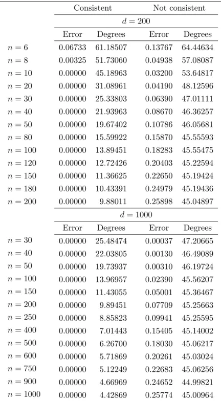
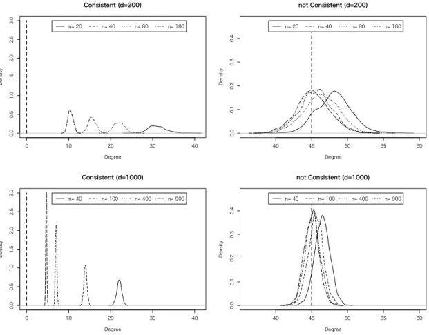
6.1 Simulation I – Discriminant Direction and Misclassiﬁcation Rate in 2-class

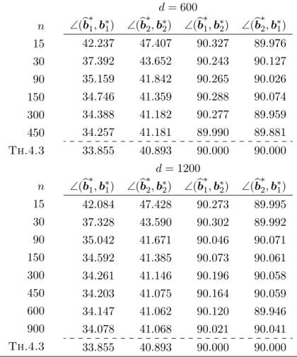
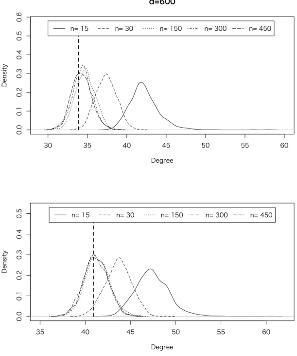
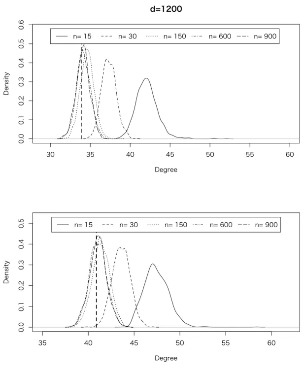
In Simulation I, our interests focus on the misclassiﬁcation rate W1(bg, θ), and the angle