np p πθπθπ 1E{()()}2(')''(') θθ  Errataforthepaper“Afamilyoftheinformationcriteriausingthephi-divergenceforcategoricaldata”anditssupplement

(1)

Unpublished document available at

http://www.res.otaru-uc.ac.jp/~emt-hogasa/, https://barrel.repo.nii.ac.jp/.

May, 2019

Errata for the paper “A family of the information criteria using the phi-divergence for categorical data” and its supplement

Haruhiko Ogasawara Otaru University of Commerce

This article gives errata for Ogasawara (2018a) and its supplement (Ogasawara, 2018b) in Sections E1 and E2, respectively. Having corrected the errors, the asymptotic results in the paper have become closer to the corresponding simulated values with increased proportions of choosing correct models by using corrected asymptotic formulas.

References

Ogasawara, H. (2018a). A family of the information criteria using the phi-divergence for categorical data.Computational Statistics and Data Analysis, 124, 87-103.

https://doi.org/10.1016/j.csda.2018.03.001.

Ogasawara, H. (2018b). An expository supplement to the paper “A family of the

information criteria using the phi-divergence for categorical data”.Economic Review (Otaru University of Commerce),69(2 & 3), 11-29.

http://www.res.otaru-uc.ac.jp/~emt-hogasa/, http://hdl.handle.net/10252/00005844.

E1. Errata of Ogasawara (2018a) Page 90, line 7: The term in (2.15)

2

2 2 2

0 0 0 0

0 0

2 2 ( )

0 0 0 0

(D)

1 E{( ) ( ) }

2 ( ') ' ' ( ')

k k

k k O n

n p

   

 

    

        

 

           

θ θ

p π

θ π θ π

(2)

2

2 2 2

0 0 0 0

0 0

2 2 ( )

0 0 0 0

2 * 2

0 0

(D)

1 E{( ) ( ) }

2 ( ') ' ' ( ')

E{( ) } E{( ) } .

k k

k k O n

k k

n p

n n p

  





 

    

 

       

 

          

 

    

θ θ

p π

θ π θ π

p π

Page 90, line 12: The term in (2.15)

2

(4) (3) 0 0 2 2 2

2 2 2 0 0

3 ( )

0 0 0

1 ( 4 2 '') E{( ) ( ) }

4 ' '

k k k O n

k

n p

    

 ^

 



  

        

θ p π

θ π

should be

2

(4) (3) 0 0 2 2 2

2 2 2 0 0

3 ( )

0 0 0

2 * 2

0 0

1 ( 4 2 '') E{( ) ( ) }

4 ' '

E{( ) } E{( ) } .

k

k k O n

k

k k

n p

n n p

    





 



 

   

         

   

θ p π

θ π

p π

Page 91, (3.1): The equation

(4) 2 (3)

2 2

2 1 0

(4) (3)

2 2 2

1 1

2 2 ''

'' 2

1 (4 2) ''(3 1)

2

K

k k

b

K K K

 

 

  

 

  

     

  



  

       



(3.1)

should be

 



  

(4) (3)

2 2 2

2 1 0

(4) (3)

2 2 2

1 1

4 3 ''

''

2 1 (8 4) ''(5 2) .

K

k k

b

K K K

  

 

  





   

     



(3.1)

(3)

1 0

1 1

{( 1)( 2) 4( 1) 4}

2

1( 1)( 2)(2 1) ( 1)(4 2) 3 1

2

K

k k

b

K K K

  



  





      

        



(3.2)

2

1 0 2

1 1

( 2) 2 1 1

2

( 1) 1( 2)( 1) 1

2

1( 1)(7 1) 8

K

k k

K K

 



 



 

        

 

 

        

 

   



should be

1 0

{( 1)( 2) 4( 1) 3} 1

( 1)( 2)(2 1) ( 1)(8 4) 5 2

K

k k

b

K K K

  



  





      

        

 (3.2)

 

2

1 0 2

( 1) 1 2 1 1

( 1) ( 1)( 1) 1

1 ( 1)(3 1).

4

K

k k

K K

 



 



 

        

 

      

   



Page 93, lines 32-34: The values “2.09”, “0.0209” and “0.8422” (two times) should be

“2.08”, “0.0208” and “0.8421”, respectively.

Page 93, line 12 from below: The term “21, 31, 39, 75 and 30” should be

“21, 41, 57, 129  and 39”.

Page 101, (A.4): The factor 2n

 on the right-hand side of the last (not first) equation of

(4)

(A.4) should be

2

 '' . Two additional terms should be inserted in

(A) (A)

  

 

  . That is, the right-hand side of the last equation of (A.4) should be

 

1 2

0 0

0 2 0

2 2

ˆ 0 0

2 ( ) ( )

1 0

2 (A) 2

1 3 3

2 3

2 3 ˆ 0 0 ( )

03 1

ˆ ( / ˆ )

2 1 2 | E{(ˆ ) ( ) }

'' 2 ˆ

ˆ ( / ˆ )

3 | E{(ˆ ) ( ) }

6 ˆ

k k

K k k k i i

k k k k

i i O n O n

k i k k p

i

i i

k k k

k k k k

i i O n

i k k p

i

p n p

i p

p

n i p n p

n

 

     

 

     



 



   

  



 

  

 







     

   

 



 



 

0 2 0

0 1

* 0

4 4

2 4

2 4 ˆ 0 0 ( )

04

3 *

1

* 2

2 *2 ˆ 0 ( ) 0

4 *

1

2 2 *2 ˆ

ˆ ( / ˆ )

4 | E{( ˆ ) ( ) }

24 ˆ

ˆ ( / ˆ )

3 | E(ˆ ) E{( ) }

1 ˆ

6

ˆ ( / ˆ )

4 |

2 ˆ

24

k k

i i

k k k

k k k k

i i O n

i k k p

i

k k k

k k O n k k

k k p

k k k

k k

p n p

i p

n p

n n p

p p n

p

 

 



     



     



  





  

 





 





  

 

   

 

 

 



0 1

* 0

2 * 2 2

0 ( ) 0

(A)

E{(ˆ ) } E{( ) } ( )

k k

k k O n k k

p

n n p O n

 

   



 



  



Page 102, (A.9): In the second term of the second line on the right-hand side of the first equation of (A.9), the factor “(2/3)” should be inserted. The factor “(3/2)” on the right-hand side of the second equation of (A.9) should be deleted. The factor

(4) (3)

2 2 2

1 2 3 ''

2  

   

 

  on the right-hand side of the last equation of (A.9) should be

(4) (3)

2 2 2

( 4 4 '') . That is, (A.9) should be

(3) (3)

2 2 3 2 2 3

2 2

2 1 0 0

2 1 1

( '') ( ) ( 2 '') ( )

'' 2 2

1 1

K

k k k

b    k    k

  





    



(5)

(3) (3)

2 2 2 2 0

2 1 0

(4) (3) (4) (3) (4) (3)

2 2 2 2 2 2 2 2

0 0

1 1

{ ( '') 2 ''} 3 2

''

{ ( 2 ) 4 2 '' ( 6 6 '')}

1 2

K

k

k k

    

 

       

 



  

         

 



        

 

   

 



 ⁽⁴⁾ ⁽³⁾ 

2 0 2 2 2 0

2 1 0 0

1 1 1

'' 3 2 4 4 '' 2

''

K

k k

k k k

     

   

    

 

           

    

 



Tables 3, 4, 6 and 8 should be as follows:

(6)

Table 3 (Corrected after publication; May 16, 2019). Added percentages of the correct (simplest) models selected by the M IC^* s over those by the ICs (the number of replications = 10,000)

The genetics of plants 3-category 4-category (Fisher, 1970; 4 categories) truncated Poisson truncated Poisson

(Bishop et al., 1975)

n: 50 200 800 50 200 800 50 200 800 The ₂ in a ICmatches the ₁ for estimation of parameters.

= 0 (G²) 2.08 .38 .13 .39 .59 .05 1.39 .31 .07

= -1 (GM²) 1.72 .41 .17 .46 .15 .01 1.38 .33 .03

= -2 (Neyman) 5.01 1.42 .27 .69 .45 .03 3.79 .80 .22

= -0.5 (T²) 1.63 .45 .09 .33 .34 .08 1.70 .17 .07

= 0.5 3.21 1.14 .26 .34 .23 .12 2.41 .54 .12

= 2/3 (C-R) 4.53 1.26 .41 .45 .20 .16 2.55 .73 .11

= 1 (X²) 5.68 1.45 .41 1.10 .18 .37 3.59 .90 .23

= 2 8.49 3.18 .85 3.19 .58 .05 6.78 1.84 .44 GJ² 2.25 .56 .12 .46 .35 .08 1.86 .28 .10

2

Eg 3.67 1.13 .24 .96 .18 .37 2.20 .65 .14 NX² 5.71 1.24 .44 .75 .89 .09 3.97 .80 .31 The MLEs (= 0) are used for all power divergences.

= 0 (G²) 2.36 .40 .22 .48 .53 .05 1.72 .37 .08

= -1 (GM²) 2.70 .46 .18 .44 .13 .00 1.75 .33 .07

= -2 (Neyman) 6.04 1.44 .34 .72 .47 .03 3.46 .85 .22

= -0.5 (T²) 2.64 .37 .07 .46 .37 .04 1.47 .32 .13

= 0.5 3.35 .78 .25 .40 .27 .11 2.63 .45 .11

= 2/3 (C-R) 5.01 .98 .19 .56 .25 .10 2.80 .54 .14

= 1 (X²) 6.39 1.37 .33 1.05 .24 .21 3.85 .81 .20

= 2 11.64 3.24 .79 3.38 .61 .06 7.13 1.84 .35

GJ² 3.18 .49 .12 .46 .37 .04 1.78 .42 .14

2

Eg 5.39 1.01 .22 .98 .24 .21 2.42 .56 .14 NX² 7.18 1.21 .36 .88 .83 .04 3.91 1.03 .33

(7)

Table 3 (Corrected after publication; May 16, 2019). (continued)

The genetics of plants 3-category 4-category (Fisher, 1970; 4 categories) truncated Poisson truncated Poisson

(Bishop et al., 1975)

n: 50 200 800 50 200 800 50 200 800 The parameter estimators by = 1 (X²) are used for all power divergences.

= 0 (G²) 2.77 .59 .12 .51 .54 .15 1.36 .31 .09

= -1 (GM²) 2.03 .49 .06 .51 .09 .01 1.62 .20 .02

= -2 (Neyman) 5.10 1.48 .35 .78 .35 .04 3.77 .76 .20

= -0.5 (T²) 1.64 .39 .14 .51 .31 .08 1.62 .27 .08

= 0.5 3.37 .86 .25 .41 .24 .17 2.39 .54 .16

= 2/3 (C-R) 4.91 1.13 .29 .57 .23 .14 2.42 .61 .16

= 1 (X²) 6.04 1.39 .30 1.12 .22 .27 3.67 .71 .19

= 2 8.68 3.33 .82 3.05 .54 .04 6.37 1.85 .55 GJ² 2.34 .57 .20 .51 .31 .08 1.73 .29 .08

2

Eg 3.99 1.10 .16 .97 .22 .26 2.29 .55 .13 NX² 5.08 1.47 .41 .80 .65 .10 3.53 .85 .17 The parameter estimators by E_g²(Eguchi) are used for all power divergences.

= 0 (G²) 2.54 .51 .11 .48 .55 .03 1.69 .31 .03

= -1 (GM²) 1.93 .50 .15 .44 .12 .01 1.54 .26 .04

= -2 (Neyman) 5.25 1.54 .26 .81 .32 .05 3.35 .86 .19

= -0.5 (T²) 1.71 .33 .16 .45 .42 .05 1.64 .27 .06

= 0.5 3.34 1.02 .29 .42 .25 .21 2.48 .55 .09

= 2/3 (C-R) 4.68 1.21 .35 .57 .24 .19 2.70 .64 .11

= 1 (X²) 6.19 1.36 .38 1.05 .21 .24 4.02 .77 .14

= 2 8.90 3.39 .76 3.32 .56 .09 7.17 1.64 .49 GJ² 2.63 .46 .19 .45 .42 .05 1.79 .34 .09

2

Eg 4.06 1.04 .23 .92 .21 .24 2.36 .55 .12 NX² 4.96 1.23 .35 .93 .80 .14 3.68 .75 .23 Note.n= the number of observations,Z= the number of deleted cases with zero frequenc(ies), NC= the number of deleted cases due to non-convergence, G² = the log-likelihood ratio statistic, GM² = the modified log-likelihood ratio statistic, Neyman = Neyman’s statistic, T² = the Freeman-Tukey statistic, C-R = the Cressie-Read statistic, X² = Pearson’s statistic,GJ²= Jeffreys’ divergence, E_g²= Eguchi’s divergence,NX²= (Neyman’s statistic +X²)/2.

(8)

Table 4 (Corrected after publication for H.A.B., b_and b^*_except the case of = 0 (G²); May 16, 2019). Simulated and asymptotic biases of the power divergences (the number of replications = 10,000)

The ₂ in a ICmatches the ₁ for estimation of parameters.

The genetics of plants (Fisher, 1970; 4 categories)

Model 1 S.B. A.B. H.A.B. S.b_ b_ S.B. A.B. H.A.B. S.b_ b_

n= 50 n= 200

= 0 (G²) -2.48 -2 -2.13 -23.9 -6.6 -2.08 -2 -2.03 -15.4 -6.6

= 2/3 (C-R) -2.61 -2 -2.22 -30.6 -10.8 -2.10 -2 -2.05 -20.1 -10.8

= 1 (X²) -2.78 -2 -2.32 -39.0 -15.9 -2.13 -2 -2.08 -25.8 -15.9

= 2 -3.78 -2 -2.88 -89.1 -43.8 -2.28 -2 -2.22 -56.9 -43.8

2

Eg -2.57 -2 -2.18 -28.5 -9.2 -2.09 -2 -2.05 -18.4 -9.2

n= 800 (b_^*)

= 0 (G²) -2.00 -2 -2.01 1.7 -6.6 (-7.0)

= 2/3 (C-R) -2.00 -2 -2.01 -.2 -10.8 (-13.7)

= 1 (X²) -2.01 -2 -2.02 -4.3 -15.9 (-19.0)

= 2 -2.04 -2 -2.05 -29.0 -43.8 (-43.0)

2

Eg -2.00 -2 -2.01 2.4 -9.2 (-13.0)

Model 2 n= 50 n= 200

= 0 (G²) -4.82 -4 -4.24 -40.9 -12.0 -4.11 -4 -4.06 -22.1 -12.0

= 2/3 (C-R) -3.94 -4 -4.47 3.0 -23.5 -4.08 -4 -4.12 -16.6 -23.5

= 1 (X²) -4.04 -4 -4.68 -2.0 -34.0 -4.13 -4 -4.17 -26.2 -34.0

= 2 -4.62 -4 -5.69 -31.2 -84.7 -4.26 -4 -4.42 -51.1 -84.7

2

Eg -3.82 -4 -4.43 9.2 -21.7 -3.96 -4 4.11 7.7 -21.7

n= 800 (b_^*)

= 0 (G²) -4.06 -4 -4.02 -46.4 -12.0 (-14.0)

= 2/3 (C-R) -4.07 -4 -4.03 -55.2 -23.5 (-27.3)

= 1 (X²) -4.08 -4 -4.04 -64.7 -34.0 (-38.0)

= 2 -4.14 -4 -4.11 -114.1 -84.7 (-86.0)

2

Eg -4.06 -4 -4.03 -51.6 -21.7 (-26.0)

(9)

Table 4 (Corrected after publication for H.A.B., b_and b^*_except the case of = 0 (G²); May 16, 2019). (continued)

The genetics of plants (Fisher, 1970; 4 categories)

Model 3 S.B. A.B. H.A.B. S.b_ b_ S.B. A.B. H.A.B. S.b_ b_

n= 50 n= 200

= 0 (G²) -6.03 -6 -6.42 -1.6 -21.0 -6.01 -6 -6.11 -2.0 -21.0

= 2/3 (C-R) -6.36 -6 -6.82 -17.8 -41.0 -6.09 -6 -6.21 -17.9 -41.0

= 1 (X²) -6.70 -6 -7.14 -34.9 -57.0 -6.16 -6 -6.29 -32.4 -57.0

= 2 -8.99 -6 -8.58 -149.3 -129.0 -6.53 -6 -6.65 -105.6 -129.0

2

Eg -6.21 -6 -6.78 -10.7 -39.0 -6.07 -6 -6.20 -13.1 -39.0 n= 800 (b_^* b_)

= 0 (G²) -6.10 -6 -6.03 -80.5 -21.0 (-21.0)

= 2/3 (C-R) -6.12 -6 -6.05 -97.5 -41.0 (-41.0)

= 1 (X²) -6.14 -6 -6.07 -112.5 -57.0 (-57.0)

= 2 -6.23 -6 -6.16 -184.4 -129.0 (-129.0)

2

Eg -6.12 -6 -6.05 -93.1 -39.0 (-39.0)

Note.n= the number of observations, S.B. = simulated bias, A.B. = asymptotic bias =2q, H.A.B. =

1 2 1

b n b ^ _   q n b ^ _, S.b_= simulated b_ n(S.B. 2 ) q ,G²= the log-likelihood ratio statistic, C-R = the Cressie-Read statistic,X²= Pearson’s statistic, E_g²= Eguchi’s divergence. The number for model identification is the number of independent parameters.

(10)

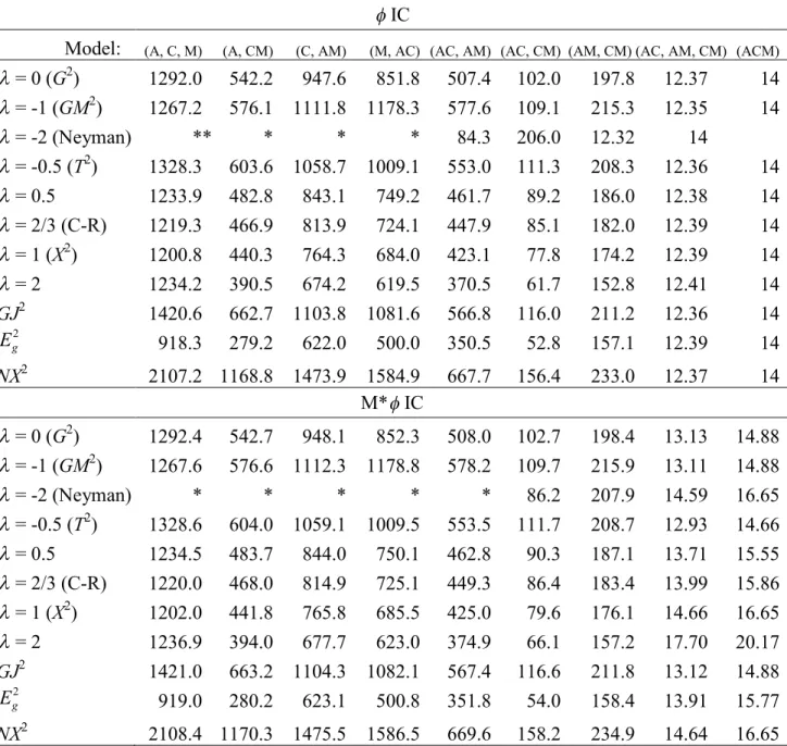
Table 6 (Corrected after publication for M*IC except the cases of = 0 (G²), = -1 (GM²), and GJ²; May 16, 2019). ICs and M*ICs of the log-linear models for the 2 2 2  table on a survey about alcohol, cigarette and marijuana use for US high school seniors

IC

Model: (A, C, M) (A, CM) (C, AM) (M, AC) (AC, AM) (AC, CM) (AM, CM) (AC, AM, CM) (ACM)

 = 0 (G²) 1292.0 542.2 947.6 851.8 507.4 102.0 197.8 12.37 14

 = -1 (GM²) 1267.2 576.1 1111.8 1178.3 577.6 109.1 215.3 12.35 14

 = -2 (Neyman) ** * * * 84.3 206.0 12.32 14

 = -0.5 (T²) 1328.3 603.6 1058.7 1009.1 553.0 111.3 208.3 12.36 14

 = 0.5 1233.9 482.8 843.1 749.2 461.7 89.2 186.0 12.38 14

 = 2/3 (C-R) 1219.3 466.9 813.9 724.1 447.9 85.1 182.0 12.39 14

 = 1 (X²) 1200.8 440.3 764.3 684.0 423.1 77.8 174.2 12.39 14

 = 2 1234.2 390.5 674.2 619.5 370.5 61.7 152.8 12.41 14

GJ² 1420.6 662.7 1103.8 1081.6 566.8 116.0 211.2 12.36 14

2

Eg 918.3 279.2 622.0 500.0 350.5 52.8 157.1 12.39 14

NX² 2107.2 1168.8 1473.9 1584.9 667.7 156.4 233.0 12.37 14

M*IC

 = 0 (G²) 1292.4 542.7 948.1 852.3 508.0 102.7 198.4 13.13 14.88

 = -1 (GM²) 1267.6 576.6 1112.3 1178.8 578.2 109.7 215.9 13.11 14.88

 = -2 (Neyman) * * * * * 86.2 207.9 14.59 16.65

 = -0.5 (T²) 1328.6 604.0 1059.1 1009.5 553.5 111.7 208.7 12.93 14.66

 = 0.5 1234.5 483.7 844.0 750.1 462.8 90.3 187.1 13.71 15.55

 = 2/3 (C-R) 1220.0 468.0 814.9 725.1 449.3 86.4 183.4 13.99 15.86

 = 1 (X²) 1202.0 441.8 765.8 685.5 425.0 79.6 176.1 14.66 16.65

 = 2 1236.9 394.0 677.7 623.0 374.9 66.1 157.2 17.70 20.17

GJ² 1421.0 663.2 1104.3 1082.1 567.4 116.6 211.8 13.12 14.88

2

Eg 919.0 280.2 623.1 500.8 351.8 54.0 158.4 13.91 15.77

NX² 2108.4 1170.3 1475.5 1586.5 669.6 158.2 234.9 14.64 16.65 Note. G² = the log-likelihood ratio statistic, GM² = the modified log-likelihood ratio statistic, Neyman = Neyman’s statistic,T²= the Freeman-Tukey statistic, C-R = the Cressie-Read statistic, X²

(11)

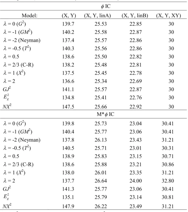
Table 8 (Corrected after publication for M*IC except the cases of = 0 (G²), = -1 (GM²), andGJ²; May 16, 2019). ICs and M*ICs of the log-linear models for the 2-way contingency table on opinions about premarital sex and availability of teenage birth control

IC

Model: (X, Y) (X, Y, linA) (X, Y, linB) (X, Y, XY)

= 0 (G²) 139.7 25.53 22.85 30

= -1 (GM²) 140.2 25.58 22.87 30

= -2 (Neyman) 137.4 25.57 22.86 30

= -0.5 (T²) 140.3 25.56 22.86 30

= 0.5 138.6 25.50 22.82 30

= 2/3 (C-R) 138.2 25.48 22.81 30

= 1 (X²) 137.5 25.45 22.78 30

= 2 136.6 25.34 22.69 30

GJ² 141.1 25.57 22.87 30

2

Eg 134.8 25.41 22.76 30

NX² 147.5 25.66 22.92 30

M*IC

= 0 (G²) 139.8 25.73 23.04 30.41

= -1 (GM²) 140.4 25.77 23.06 30.41

= -2 (Neyman) 137.8 26.13 23.43 31.21

= -0.5 (T²) 140.5 25.71 23.01 30.31

= 0.5 138.9 25.83 23.15 30.71

= 2/3 (C-R) 138.6 25.88 23.21 30.86

= 1 (X²) 138.0 26.01 23.35 31.21

= 2 137.7 26.64 24.00 32.80

GJ² 141.3 25.77 23.06 30.41

2

Eg 135.1 25.79 23.14 30.81

NX² 147.9 26.22 23.49 31.21

Note.G²= the log-likelihood ratio statistic,GM²= the modified log-likelihood ratio statistic, Neyman = Neyman’s statistic,T²= the Freeman-Tukey statistic, C-R = the Cressie-Read statistic,X²= Pearson’s statistic,GJ²= Jeffreys’ divergence,

2

Eg= Eguchi’s divergence,NX²= (Neyman’s statistic +X²)/2. In “linA”, (1, 2, 3, 4) '



u and v(1, 2, 3, 4)', and in “linB”, u(1, 2, 4, 5) ' and



(12)

E2. Errata for Ogasawara (2018b)

Page 12, line 2: A comma should be inserted. That is, the right-hand side of the third equation of (S.1)

1 1

0( 1) 0( 1) 0( 1) 0( 1) 0 ( 1)

{diag( _K_ ) _K_ _K_ '}{diag (^ _K_ ) ^_K _K_ }

 π π π π  1

should be

1 1

0( 1) 0( 1) 0( 1) 0( 1) 0 ( 1)

{diag( _K_ ) _K_ _K_ '}{diag (^ _K_ ), ^_K _K_ }

 π π π π  1 _.

Page 18, (S.12): The symbol

2

( , , )i j k on the right-hand side of the first equation of (S.12) should be

3

( , , )i j k ^.

Page 19-20, (S.14): The factor m a b k k₄( , , , )(two times) in (S.14) should be

2

4 0 0 0 0

{ ( , , , ) (m a b k k   _ab _aa  _a _b)( _k  _k)}. That is, (S.14) should be

2

0 3

1 , 1

2 0

(A) (B)

( ) ( ) ( ) 0 4

, , 1

(B) (3)

2 2 0 3

2 1

0

0 , 1

''

2 1

( 2 ) ( , , )

'' 2

1 {2( ) 2( ) 2( ) 6 } ( , , , )

6

1 ( '') ( ) ( , , )

2

1 ( 2 )

2

K K

ka kb k

k k a b

K

K ka K kb K kc k

a b c

K

ka k

k a

K

ka kb k

a b

b a b k

m a b c k

a k k

    

 



    



  



 



 

      

 

    

   

   

 



I I I

4

2

0 0 0 0

{ ( , , , )

( _{ab aa} _a _b)( _k _k)}

m a b k k

      ^

   

 ^(S.14)