KoujiIshii e LinearCollider AStudyofCalorimeterforFuturee

March 6, 1995

A Study of Calorimeter

for Future e e

Linear Collider

Kouji Ishii

Master’s Thesis,

Department of Physics, Faculty of Science, Kobe University, Rokkodai, Nada, Kobe 657, Japan

Abstract

As a program of R&D for the JLC experiment, we constructed test modules of compensating Pb-scintillator fiber calorimeter for detection of electromagnetic and hadronic showers. Using these test modules we performed a beam test at KEK PS 2 beam line. We also tested three types of photon detection devices in strong magnetic field. In this article I report results of these two tests.

Contents

1 Introduction 3

2 JLC Experiment 3

2.1 Physics

3

2.1.1 Top Quark

4

2.1.2 Higgs Boson

6

2.1.3 Supesymmetric Particles

7

2.2 Detector

8

2.3 Calorimeter

9

3 Tests of Prototype Calorimeter 10

3.1 Test Modules

11

3.2 Setup of the Beam Test

12

3.3 Analysis

13

3.3.1 Energy Resolution for Electrons

13

3.3.2 Position Resolution for Electrons

14

3.3.3 Energy Resolutions for Pions

15

3.3.4 Electron Identification

16

3.4 Discussion

19

4 Tests of Photon Detection Devices 21

4.1 Photon Detection Devices

21

4.2 Setup in Strong Magnetic Field

22

4.3 Results

23

4.3.1 FMPMT

23

4.3.2 HPD

24

4.3.3 VAPD

24

4.4 Discussion

25

5 Conclusion 25

Acknowledgment

APPENDIXES

A Calorimeter 27

A.1 Principle

27

A.2 Definition of the

and

29

A.3 Compensating

31

A.4 Examples

32

B Algorism 33

B.1 Thrust

33

B.2 Acoplanarity

33

C Comparison 34

C.1 Performance of Compensating Pb-scintillator Calorimeter

34

C.2 Performance of Pb-scintillator Fiber Calorimeter

35

1 Introduction

Towards 21st. century, electron-positron linear colliders with central mass energies in TeV region are being planned. In these projects, a rich physics will be expected and we can study not only the Standard Model but also new physics beyond the Standard Model. JLC is one of these projects. I have participated to this project and studied the calorimeter with other collaborators.

The calorimeter is a device to detect total energy of shower particles ( see Appendix A ). It is one of main detector components in collider experiments. In future electron-positron linear collider experiments, it is essential to have a hermetic detector with super energy resolution. From this requirement, the calorimeter must have good energy resolution for both electromagnetic and hadronic shower profiles and it is desirable to be located inside solenoid. One of the solutions to achieve good energy resolution is compensating Pb-scintillator fiber calorimeter ( see Appendix A.3 ). We constructed test modules and made a beam test at the KEK PS

2 beam line. We also tested three types of photon detection devices in strong magnetic field in order to read out signals from the calorimeter inside solenoid. In this article I introduce the JLC experiments and report results of these two tests.

2 JLC Experiment

In the JLC-I ( Japan Linear Collider phase 1 ) report [1] published in 1992, it has been proposed to construct the linear collider of center mass energy 300-500 GeV as early as possible. In this section I briefly introduce physics motivations of JLC-I and a detector proposed for the experiment.

2.1 Physics

At this energy region following particles, if they exist, can be detected and studied in detail.

top quark (

¯

)

a ( light ) neutral Higgs boson (

)

other neutral Higgs bosons (

or

or

)

charged Higgs bosons (

)

supersymmetric particles (

˜

˜

or ˜

˜

)

The inside of the bracket is a dominant production at the JLC-I experiment. For neutral Higgs bosons,

means a particle expected from the Standard Model or the extension of it and

0 ^! 0 ^"

and

mean the particles coming out from the model of Minimal Supersymmetric

extension of the Standard Model. The ˜

and ˜

are the chargino and slepton particle. The detail

is mentioned in later section. Through the search and study of the above particles, we can test

the Standard Model with super precision and may be able to test supersymmetry ( SUSY ).

Even if the light neutral Higgs boson can not be detected at the JLC-I experiment, we can get the Higgs mass bound through the radiative correction with super precision measurement of the

and

(

1

and

20

) due to superior luminosity (

576

5

10

). The absence of the light Higgs boson implies the death of low energy SUSY and GUT. In this case, we might be able to suggest a new physics through the measurements of anomalous couplings in self-interactions of vector bosons (

and

). These studies will also open up the possibility to get insights into physics at higher energy scale.

Besides, we can study CP violation and flavor mixing through investigating

physics on the

pole. The studies of CP violation and flavor mixing are not only to test the Standard Model but also very important to probe underlying physics at very high energies. Due to some superior performances of JLC accelerator ( high luminosity, highly polarized electron beam, and narrow beam ) and large production cross section of

mesons on the

pole, the JLC-I experiment has some advantages in comparison to the other experiments.

Thus, a large number of physics are expected, we might be able to test physics of the beyond Standard Model. This is the reason for us to look forward to early realization of the JLC-I experiment.

In the next subsections, I give outlines of the physics and show the way of detecting top quarks and Higgs bosons. Both particles are missing in the Standard Model at present, the study of them are main theme of the JLC-I experiment. I also indicate how to detect supersymmetric particles.

Here, I emphasize the detection of these new particles largely depends on the performance of the detector.

The other arguments or details are described in Ref. [1].

2.1.1 Top Quark

The top quark must exist and is no heavier than 200 GeV from analyses of the electroweak radiative corrections. ( Ref. [3] )

%)&=->%@?BAC%)(DA

200

In April 1994, the the Collider Detector at Fermilab ( CDF ) group reported the first ”evidence”

for top quark production at the Fermilab Tevatron collider (

¯ collisions,

= 1.8 TeV ) in Ref. [4]. They searched for 2-jets and 4-jets events associated with electron or muon. Total 12 events are found with an integrated luminosity of 19.3 pb

. They estimated a top quark mass of 174

10

12

GeV/c

and the

¯ production cross section was measured to be 13.9

4^H8

pb.

This value of the top quark mass is consistent with the expected value from the electroweak measurement of LEP experiments ( 177

11 18

191

GeV/c

Ref. [5] ). But in

¯ collisions, it is too difficult to study detailed features of the top quark, and it will be first performed with e

e

linear collider in detail.

At JLC-I, we can easily observe

¯ pair production. In that region ( 150

200 GeV ) the top quark decays mainly to

. The

boson decays into

¯ or

¯ and the final states of the top quark are classified to the following three cases.

1The secondary errors are caused by changing the Higgs mass from 60 GeV to 1 TeV.

6-jets (45 % )

4-jets + 1 charged lepton (44 % )

2-jets + 2 charged leptons (11 % )

As an example the first case ( 6-jets ) is considered. In order to select the top quark events from the backgrounds, we applied the following requirements.

conservation of 4-momentum

6-jets at the final states

two pairs of jets whose reconstructed invariant mass equal to

small thrust ( see Appendix B.1 )

Fig. 1 ( quoted from Ref. [3] ) shows the thrust distributions after the all events selections exclusive of the thrust cut with the Monte Carlo Simulation. It is clear that the thrust cut is efficient for

¯ selection. In this case, a detection efficiency is 26 % and the signal to background ratio exceeds 10.

The top quark we are going to deal with has many unique features, compared to quarks of other flavors. This is primarily due to its large mass and width. The decay of the heavy top quark is dominated by

, and it causes the large width due to the mass difference of W and t (

%)(TS %,&

). Because of it’s large width, the top quark decays before the non-perturbative part of the potential effect it. Thus, the large width prevents this potential from affecting the threshold calculation, uncontrollable theoretical ambiguities are absent from the

¯ system. This implies that we can perform the clear test of perturbative QCD with measurement of the cross section in the whole threshold region ( threshold scan ). Experimentally, the parameters that enter the threshold cross section;

) may be determined by the threshold scan. Fig. 2 ( quoted from Ref. [3] ) is an example of the energy scan to determine

and

Z [

Vb%

? ^

.

On the other hand, the momentum distribution of the top quark reflects the shape of the

¯ potential that it probes. The momentum distributions provides additional information on

,

X (

, and

. Fig. 3 ( quoted from Ref. [3] ) is an example of the reconstructed momentum distributions at the

¯ threshold. The measurement of the forward-backward asymmetry is also used with the determination of the

and

.

Besides, there is another new and remarkable property of a heavy top quark; the heavy top will decay before forming a top-hadron. This enable us to measure the helicities of parent quarks by angular analyses of their decay daughters. The helicity measurement will provide us with a powerful tool to systematically investigate the top quark production and decay vertices, in particular, when the vertices involve new particles expected in the SUSY scenario.

A lot of studies about the top quark are expected in JLC-I. We have to do a intensive tests of

the Standard Model through the above precision measurements.

2.1.2 Higgs Boson

At the present, the Higgs boson or Higgs mechanism expected from electroweak theory have not been experimentally discovered and lower limit on the mass of the Standard Model Higgs particle is 64.5 GeV at 95 % confidence level ( Ref. [6] ). The Higgs boson does not have a strong confine such as the top quark in the Standard Model framework. But assuming the GUT, Higgs mass does not exceed 200 GeV( Ref. [1] [2] ), and the light Higgs boson can be searched easily by the process;

at the JLC-I experiment. Especially, a search of intermediate Higgs boson

2

is important because it is too difficult to detect such a intermediate Higgs boson at the other experiments. The LEP-II experiment is limited by the center of mass energy and the LHC experiment or other hadron collider do not have a good observable decay mode. On the other hand, the heavy Higgs boson

2

will be searched for using the process;

4

at future hadron colliders ( LHC ).

In the Minimal Supersymmetric extension of the Standard Model( MSSM ), the Higgs sector consists of two doublets, resulting in five physical particles; two CP-even scalars, i.e. a light one (

) and heavy one (

), one CP-odd scalar (

), and a pair of charged Higgs (

). There are relations among the masses of these particles. The

,

, and

can be given in terms of

and tan

, where tan

is the ratio of the two vacuum expectation values of two Higgs doublets. The Higgs phenomenology in the MSSM is either the production of only the light Higgs particle with a cross section similar to that of the Standard Model Higgs particle

V\%

hji

150

or the simultaneous productions of

, and

(

150 GeV ). In any case, we can discover at least one Higgs particle at JLC-I if nature is really under the GUT condition.

Owing to the mass contribution of coupling to Higgs boson, the decay branching ratio is dominated by

¯

L

in case of

140 GeV, while in case of

140 GeV the

0

;mc;n

decay mode is dominant. Here, we consider the main decay mode is

¯

. Depending on the decay modes of

, event topologies of the process

are classified into the next three.

0 0

L

¯

L

(

10 % )

0 0

oN ^NL

¯ ¯

(

70 % )

0 0

Q

¯

Q L

¯

L

(

20 % )

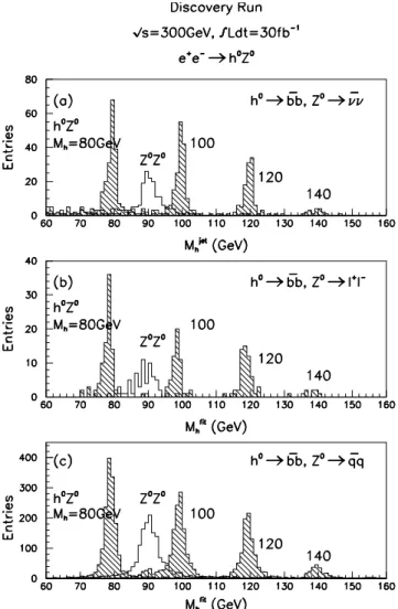
A typical event of each topology is shown in Fig. 4 ( quoted from Ref. [2] ). The signals of Higgs boson will be observed as a peak in the invariant mass distribution of 2-jets, requiring the invariant mass of the rest system ( 2 leptons , 2-jets, and missing of the 4-momentum ) consistent with m

. The main backgrounds come from the following processes.

$o;n;

$

0

0

$o Q ;

The background of

and

have a peak at the forward direction in differential cross sections. The

and

events do not include

-quarks at final states. Thus, to select Higgs bosons we required of events produced in central region with

-quarks. Fig. 5 ( quoted from Ref. [2] ) shows the reconstructed

at an integrated luminosity of 30 fb

( correspond

100 days running ).

Once a Higgs particle is discovered, a detailed study should come next. The question to be answered is whether the Higgs sector is that of the Standard Model or not. Precise measurements of the production cross section, the decay width, and the decay branching ratio of

will answer this question. Fig. 6 ( quoted from Ref. [2] ) shows the contours of the total width of the MSSM Higgs in the

and tan

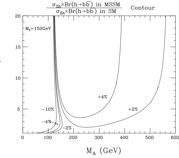
plane. We can also establish the non-minimality of the Higgs boson by measurement of the total cross section of

(

) and the branching ratio (

<rsV 0

oL

¯

Lt^

). We should compare the

¯

L^

of the measurement with that of the Standard Model. It is shown in Fig. 7 ( quoted from Ref. [2] ). The decay channel of

is also interesting. For the Standard Model this branching ratio is

10

, but it can be

10

or much smaller for large tan

and relatively small

in the MSSM. Whether we can achieve this study or not much depends on the performance of the calorimeter. The good energy resolution for

( electromagnetic shower ) is required because the only calorimeter can detect

directly.

The Higgs studies also provide us a possibility to probe higher energy scale physics through the mass ratio of the bottom quark to the tau lepton. At present, large theoretical error on

from

¯

L

potential prevents us from making a precise test of the GUT predictions. However, if the mass of the Higgs boson is in the region where the main decay mode is

¯

, we can make a precise measurement of the

-quark mass by measuring the branching ratio for

¯ . In any models which generate the

-quark and

lepton masses from the same Higgs doublet, the ratio of the branching fraction for

¯

L

and

¯

is completely fixed up to the ambiguities in

%)v

and

. Fig. 8 ( quoted from Ref. [2] ) shows contours of the branching ratio for

¯ in the plane of

and

.

The detection of one or more extra-Higgs bosons;

,

, and

is the direct evidence of the non-minimality of the Higgs sector expected in the SUSY models. The processes of the production were already shown (

and

). The detection of the

process is similar way with the light Higgs boson. A detailed studies of the others are reported in Ref. [1], [2] and [7]. In any case, the detection at the JLC-I is easy.

As we described above, we can perform discovery of the intermediate Higgs boson, if it exist.

In this case we may be able to test the SUSY with the precision measurement of the Higgs properties or the direct search for the other Higgs bosons.

2.1.3 Supesymmetric Particles

The SUSY predicts the existence of a light neutral Higgs boson whose discovery at JLC is easy, as described in the previous section. However the discovery and study of the lightest neutral Higgs boson alone is not enough to prove the SUSY. It is definitely necessary to discover at least one supersymmetric particle. There are a lot of chances to discover at least one supersymmetric particle.

In the framework of Supergravity models with the conditions of the GUT the following

the parameters; (

tan

), which determined the mass spectra and the interactions of supersymmetric particles, are involved ( Ref. [8] ). In order to avoid unnecessary complications we will make the following simplifying assumption. The R-parity is exactly conserved which implies that supersymmetric particles can only be pair-produced and the Lightest Supersymmetric Particle ( LSP ) is absolutely stable. And the LSP might be the light neutralino to be consistent with cosmology. We further assume that the supersymmetric particle in question is the lightest charged supersymmetric particle.

Under these assumptions, the lighter chargino or the right-handed slepton will be the first observed supersymmetric particle at the JLC-I. The following decay modes of the chargino and slepton are some observable modes. Dominant decay modes of these particles are listed below.

˜

˜

˜

˜

˜

¯

˜

˜

˜

˜

#

˜

0 0

where ˜

is the lightest neutralino ( in this case LSP ) and

can be any of

,

, and

.

In any case, we can use a missing transverse momentum or a large acoplanarity ( see Appendix B.2 ). The main backgrounds ( example

) are removed by this acoplanarity cut.Fig. 9 ( quoted from Ref. [2] ) shows an example of the acoplanarity distribution for the 2-jets + 1 lepton ( one chargino decays hadronically and the other decays leptonically ) final states from the lighter chargino pair productions with the Monte Carlo simulation. The energy distributions of the 2-jets systems from the lighter chargino decays and of the muons from smuon are shown in Fig. 10 ( quoted from Ref. [2] ) and Fig. 11 ( quoted from Ref. [2] ), respectively.

These figures explicitly show that we can search for a supersymmetric particle at the JLC-I experiment. In order to detect the missing

, we require a good angular coverage and we must construct the hermetic calorimeter.

2.2 Detector

In order to achieve the physics goals of the JLC-I experiments, we need a hermetic detector with super energy/momentum resolution, good b-tagging capability and good lepton identification capability. We made a conceptional design of the detector taking account of the physics simulations as well as the experience of previous experiments and R&D programs. An apparatus proposed by the JLC working group is shown in Fig. 13( quoted from Ref. [1] ). The detector is based on modest extensions of the presently available technology. The parameters and the performances of each detector component are summarized in Table 1( quoted from Ref. [1] ).

These values were assumed in the previous physics simulations. Except muon detector ( MUON

), three detectors; namely vertex ( VTX ), central drift chamber ( CDC ), and calorimeter ( CAL

) are placed inside 2 Tesla superconducting solenoid to achieve a hermetic structure and good

energy resolution.

DETECTOR

TYPE CONFIGURATION PERFORMANCE VTX

CDC

CAL

MUON

( Vertex Detector )

( Central Drift Chamber )

Silicon CCD

Small-cell Jet Chamber

Lead + Plastic Scintillator Sandwitch

( Compensated )

Pixel Size ; 25 µm

Layer Position ; r=2.5cm & 7.5cm Thickness ; 500 µm / layer

| cos θ | < 0.95

Position Resolution ; σ = 7.2 µm Impact Parameter Resolution δ [µm];

δ = 11.4 + (28.8/p) / sin θ^{2 2 2 3} Radius ; r = 0.3 - 2.3 m

Length ; l = 4.6 m Number of Sampling = 100

| cos θ | < 0.70 ( full sampling )

Position Resolution ; σ = 100 µm ( / axial wire ) σ = 2 mm ( / stereo wire )^xz Momentum Resolution ;

σ / Pt = 1.1x10 Pt + 0.1%_Pt ^-4

EM part ; thickness = 29 Xo cell size = 10cm x 10cm HAD part ; thickness = 5.6 λo

cell size = 20cm x 20cm Si Pad ; pad size = 1cm x 1cm

| cos θ | < 0.99

Energy Resolution ;

σ / √E = 15% / √E + 1% ( e & γ )_E σ / √E = 40% / √E + 2% (hadron)E Si Pad Position Resolution ; σ = 3 mm Si Pad e/π Rejection = 1/50

Single Cell Drift Chamber

Number of Superlayers ; 6

| cos θ | < 0.99

Position Resolution ; σ = 500 µm Pt > 3.5 GeV ( barrel )

* All momentum and energy are expressed in [ GeV ].

Number of Layers ; 2 layers

| cos θ | < 0.95 ( 20 samplings ) σ / Pt = 5 x10 Pt + 0.1%_Pt ^-5 ( with vertex constraint )

Table 1: Parameters and performances of the JLC detector. ( This table is quoted from Ref.[1]. )

2.3 Calorimeter

The following items show the requirements of the calorimeter at the JLC-I.

1 good energy resolution for electromagnetic shower:

15%

1%

2 good energy resolution for hadronic shower:

40%

2%

3 good position resolution for electromagnetic shower:

several mm

E

4 good identification of electrons from hadron backgrounds: a pion rejection factor of about 50 for an electron efficiency of 90 % (the pion rejection factor is defined in section 3.3.4)

5 hermetic calorimeter

where energy E is given in GeV. The values are expected to be achieved by a modest extension of current technology. We can detect the high energy neutral particles such as

s,

s and neutrons (

) only by the calorimeter.

s decay into two

s immediately after these production.

is important in the case of studying

2

s ( see section 2.1.2 ). This branching ratio is

10

even if the Standard Model. The mass of Higgs boson from two

s is described as

%

2 ⁶

%

2^{‰M‰ 6}

2

‚

2^V

1

Therefore, the performance of the energy and position resolution for electromagnetic shower is a main key of that study. The process of

¯

L

also need good energy and position resolution for electromagnetic showers. Because

radiates

by bremsstrahlung in the CDC, the recoil mass of the

is depending on the resolution.

A ( hadron ) jet contains about 20 % neutral hadrons (

,

). In order to calculate invariant mass of two or several jets, we also need good energy resolution for hadronic shower. As an example, we show Higgs mass resolution in the the

process. In Fig. 12 ( quoted from Ref. [1] ), the result of a simulation of the di-jet mass resolution, assuming the performances listed in Table 1 and smeared according to the resolution, is presented. The value of

= 4 GeV is reasonably good jet mass resolution and it shows a great capability to separate reconstructed Higgs bosons from the backgrounds ( mainly Z particles in the

process ) at a few GeV level.

The electron identification is important in many cases. An example is to search for events of

¯

L

or of top quark associated with the electron. The reason for necessity of hermetic calorimeter is to measured missing energy. In chargino or slepton pair production, a LSP is emitted and carries non-negligible energy, resulting missing energy.

In the Table 1, we chose a compensating Pb-scintillator calorimeter ( sandwich type ) which is one of the solutions. Combination of Pb and scintillator has the potential for compensating calorimeter, which has good energy resolution for hadronic shower ( see Appendix A.3 ). By the calculations of R. Wigmans [10], our requirement for hadronic showers ( 40%

) can be achieved with the configuration of Pb=10mm and scintillator=2.5mm. For electromagnetic showers, it is able to achieve our requirement( 15%

) with the configuration of Pb=4mm and scintillator=1mm by the simulation studies of Y. Fujii in Ref. [11]. Experimentally, ZEUS groups [12] have reported the performance of the compensating Pb-scintillator calorimeter. These studies and results are summarized in Appendix C.1.

On the other hand, the compensating Pb-scintillator fiber calorimeter is one of the other solutions and it has some advantageous performances compared with sandwich type. It is described in next section.

3 Tests of Prototype Calorimeter

2

To achieve the energy resolution of JLC calorimeter we choose compensating Pb-scintillator fiber calorimeter. Because of the fine sampling frequency, fiber calorimeter has better energy resolution than other Pb-scintillator calorimeters such as sandwich calorimeter made of Pb plates, scintillator plates, and wave length shifter bars. Moreover, it is possible to reduce dead space, which might be occupied by wave length shifters in case of sandwich type. The better position resolution can be achieved if the read-out cross section is small. Several groups [14] [21] [22] [25] [27] have reported the excellent performance of the Pb-scintillator fiber calorimeter. These performances are summarized in Appendix C.2.

As a program of R&D for the JLC experiments, we constructed test modules of Pb-scintillator fiber calorimeter. We made a beam test of the modules at KEK PS

2 beam line to test the

2The content of this section will be submitted as a paper.

following items.

energy resolution for electrons and pions

signal ratio of electrons to pions(compensation)

linearity of the signal

position resolution for electrons

identification of electrons from pions

angular dependence of both energy and position resolution for electrons

The angular dependence of both energy and position resolution for electrons is due to lateral shower spread. For Pb-scintillator fiber calorimeter, the beam direction is almost parallel to the fiber direction. Because the electron shower spreads only a few cm and ratio of active layer to absorber in the shower is fluctuated by incident position and angle. Thus, both energy and position resolution depend on the angle and at the small angle (

0

) the resolution may be worse. Therfore, we test their effects experimentally.

Due to the limit of the beam energy ( 4 GeV ), response of the modules only to low energy particle could be tested.

3.1 Test Modules

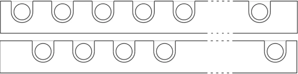
We constructed test modules of compensating Pb-scintillator fiber calorimeter. The schematic view of the test modules are shown in Fig. 14. The volume ratio of lead to fiber was set at approximately 4:1 in order to achieve the compensation. For structural hardness the Pb plates contained 6% antimony in weight. A Pb-plate was 10 cm wide and 130 cm long 2 mm thick ( 173

and 6.2

; see Appendix A.2 ), and had machined grooves for the fibers on its upper side ( see Fig. 15 ) with 2.2 mm pitch. The fibers were 1 mm

and made of polystyrene-based scintillator KURARAY SCSF-38. The polystyrene core and PMMA clad had refractive indices of

1

59 and

1

49, respectively. The surfaces of fibers were painted with white reflector in order to increase light yield. The attenuation length of scintillation light was measured to be roughly 300 cm.

The Pb-plates filled with scintillation fibers in their grooves were stacked to form a test module material with dimension of 10

5

130

. Because of thickness of the reflector, twenty two or three Pb plates were stacked in the height of 5 cm. At rear end the fibers were grouped into two segment and bundled. The edge of each bundle was cut to make a flat surface and polished. The bundle was glued to an acrylic light guide and viewed by a photomultiplier tube ( Hamamatsu R1335 ). At the front end the edges of the fibers were polished and painted with white reflector. A total of eight modules were constructed and sixteen channels were read out. They were arranged to have a cross section of 20

20

as shown in Fig 14. All modules were inserted into a box made of 7 mm stainless steel. It was used as support structure and light shielding.

In addition, we constructed a special test module which had a light guide and a photomultipliers

at each end. This module was used to study electrons/pions separation from timing properties of

signals at both ends.

3.2 Setup of the Beam Test

Tests of the calorimeter modules were performed at the

2 beam line of the KEK-PS. The maximum momentum available was about 4 GeV/c. The electron/pion ratio in the beam was about 1/1000.

Fig 16 is the schematic view of the setup for the beam test. We set two trigger counters ( S1,S2 ) in front of the movable stage where the calorimeter modules were mounted. Each of them was a scintillation counter with a cross section of 5

5 cm

, and the distance between the two counters was about 280 cm. There were two gas ˇ Cerenkov counters ( C1,C2 ) between the trigger counters to identify electrons and pions. To take electron data the coincidence of S1,S2,C1 and C2 signals were required, while only the coincidence of S1,S2 signals were required for pion data. The electron contamination in the pion data were later removed in the offline analysis.

In order to precisely measure the incident position of the particles, we set two drift chambers ( DC1,DC2 ) between S2 counter and the movable stage. Each of them had readouts for vertical and horizontal position, respectively. The cross section of the drift chambers were 20

20 cm

, and the position resolution was about 2 mm at the front surface of the test modules.

In addition to the test modules, following detectors were mounted on the movable stage.

The leakage shower counters which surrounded the test modules (see Fig 17). The counters were sandwich-type calorimeter consisting of scintillator plate ( 2.5 mm thick ) and lead plates ( 10 mm thick ), compensating too. The scintillation light was lead into two photomultipliers through two wave length shifter plate of 2 mm thickness. The active volume of a module was 38.5

18.6

100 cm

in size.

The preshower detector in front of test modules ( upper stream ). The preshower detector consisted of six layers of a scintillator plate ( 1 mm thick ) and a lead plate ( 4 mm thick ), resulting in 4

. These preshower detector were also compensating. The scintillation light was lead into four photomultipliers through two wave length shifter plates of 4 mm thickness.

The silicon-pad detector between the preshower detector and the test modules. The silicon-pad detector consisted of 216 pads ( PIN silicon diodes made in HAMAMATU ), one pad was 300

m thickness and 10

15 mm

in size, total active area was 18

18 cm

. This detector was set to test the position resolution for electrons and the separation of electrons from pions through the preshower detector. In this paper we did not use the data of the silicon-pad detector.

All the detectors, namely the test modules, the leakage shower counters, the silicon-pad detector and the preshower detecter, were mounted on a movable stage. The stage could move horizontally and vertically, as well as rotate in the horizontal plane so that the incident angle of the beam to the test modules could be changed.

All the signal from the calorimeters were fed into 12 bit ADCs. The ADC channels had two different ranges to have an effective dynamic range of 15 bit. The signals of the drift chambers were fed into 15 bit TDCs ( same bit type as the ADC ) where one bit corresponded to 100 ps.

Once an event was triggered, all the data were taken by a personal computer ( NEC PC98NSR ).

In special runs to take the pulse shape, the signals from the calorimeters were fed into a digital oscilloscope of 2 GHz sampling. The data were transferred to the personal computer.

We took various data changing the setup of the beams and the detectors. The momentum of the beam was set of 1.0 , 1.5 , 2.5 and 4.0 GeV/c. The incident position and angle to the test modules were changed with the movable stage. The data without the preshower detector were also taken.

3.3 Analysis

In the following analysis, only single-track events were used. They were selected with the conditions given below.

The pulse height of each trigger counter ( S1 and S2 ) is consistent with that of a signal minimum ionizing particle. Fig. 18 shows typical pulse height distributions of the trigger counters.

There was one and only one hit in each drift chamber ( DC1 and DC2 ).

The gain of each channel in the test modules was calibrated with using the electron data to the central region ( 2

2 cm

) of each segments with an incident angle of 3

in the horizontal plane (

3

). By D. Acosta, et al. ( Ref. [14]), the angular dependence of the energy resolution is flat at

3

. The electron energies were 1.0, 1.5, 2.5, and 4.0 GeV. The response was found to be linear in the relevant energy range. The leakage shower counters were calibrated in a similar way. The energy resolution of the leakage shower counters for electrons was found to be

24

0%

0

4%.

The results were compared with Monte Carlo simulation based on GEANT3. The detail is described in Ref. [9].

3.3.1 Energy Resolution for Electrons

To evaluate the energy resolution for electrons we use only the events where electrons hit the center ( 2

2 cm

) of each segments. The total energy of the test modules (

) was calculated as the sum of the signals of all the 16 channels. In case the preshower detector ( PSD ) was located in front, the total energy (

) is calculated with the following formula

‚ 6 Z 8

‚œ›

–”

ƒ‚

‡ € hž”c•\–—™˜!šŸ˜

where

is the energy deposit measured in the preshower detector. The coefficient

was determined at each energy point to obtain the best energy resolution. For the data without the preshower detector,

is simply used as the total energy. An example of the total energy distribution is shown in Fig. 19.

By fitting the total energy distribution to a Gaussian function, we obtained the energy resolution.

The results at

3

with and without the preshower detector are given in Table 2 and also

shown in Fig. 20. The resolutions can be expressed by the following formula.

U

‚ 6

14

4

1

63%

¡ ‚

V¢/41£^

ƒ

0

15

1

03% with PSD

6

15

2

1

37%

¡ ‚

V¢/41£^

Š

0

58

0

82% without PSD

Energy 1 GeV 1.5 GeV 2.5 GeV 4 GeV

w/ PSD 13.8

0.87 12.6

0.76 9.45

0.50 7.23

0.35 w/o PSD 13.4

0.78 12.5

0.75 9.53

0.31 6.81

0.24

Table 2: Energy resolution

(%) for various energy.

The angular dependence of the energy resolution was studied with 2.5 GeV electrons at

4

6

0

1

2

3

6

and 9

. Fig. 21 shows the results of the energy resolution as a function of the incident angle

. Although the angular dependence is not seen clearly, we observed slightly worse energy resolution at

0

. We think a reson for the indistinct angular dependence is due to the low beam energy.

3.3.2 Position Resolution for Electrons

The incident position can be obtained from the test modules. The position (

) weighted by the energy is calculated as

¤

6§¦]¨4¤

¨‚ ¨

¦@¨

‚ ¨

¥ 6 ¦ ¨ ¥ ¨‚ ¨

¦ ¨ ‚ ¨

where (

) and

are the center position and the energy deposit of

’the channel. In this analysis the data without the preshower detector is used. Fig. 22 shows the scatter plot of the incident positions measured by the drift chambers and the position derived from the above formula, where the electrons of 4 GeV energy were incident with a horizontal angle (

) of 3

to the test modules without the preshower detector in front.

Using these plots and assuming that the positions measured by the drift chambers are correct, we can get functions for further correction. We used the tangential function here. We show the distribution of the difference of the corrected position and the position measured by the drift chambers in Fig. 23. The distributions are fitted to Gaussians, and the resolutions are calculated.

The results at

3

are summarized in Table 3 and shown in Fig. 24. The relation between the

position resolution and electron energy can be expressed as

U  6

6

2

0

3

¡ ‚

V¢/41.^

ƒ

0

6

0

2

3

U™°

6

4

7

0

3

¡ ‚

V¢/41.^

ƒ

1

4

0

2

3

The difference of the behaviors between the

-coordinate and the

-coordinate is considered to be due to the difference of the beam spot at the various beam energy. The position resolution depends on the incident point and at the edge of one segment the test modules have better resolution because we can get more information about the incident point from the adjacent channels.

The angular dependence of the position resolution is studied with the data of 4.0 GeV electrons at

0

3

6

and 9

. Fig. 25 shows the results of the energy resolution as a function of the angle

. The angular dependence was not seen.

3.3.3 Energy Resolutions for Pions

We use the pion data with incident angle of 0

for the energy resolution for pions. The contamination of electrons in the data is removed offline using the information of ˇ Cerenkov counters. We calculate the total energy as the sum of all the signals from the test modules and leakage shower counters. Similar to the case for electrons, if the preshower detector was located in front,

is further added to the total energy. An example of the total energy distribution is shown in Fig. 26. The energy resolutions at each energy points are listed in Table 4. They are also shown in Fig. 27.

U

‚ 6

31

5

1

79%

¡ ‚

V²/01.^

ƒ

9

06

1

19%

U

‚ 6

30

1

1

82%

¡ ‚

V²/01.^

ƒ

7

45

1

15%

The large constant term reproduced by the simulation [9]. It may be caused by the further shower leakage for pion from the test modules and leakage shower counters. Because of serious problem at high energy, we want to check it experimentally by locating further leakage counters.

Energy 1 GeV 1.5 GeV 2.5 GeV 4 GeV

x 6.94

0.13 5.33

0.12 4.37

0.10 3.74

0.09 y 6.52

0.16 4.97

0.11 4.45

0.09 4.12

0.09

Table 3: Position resolution

(mm) for various energy.

Energy 1 GeV 1.5 GeV 2.5 GeV 4 GeV w/ PSD 40.29

1.03 35.12

0.61 28.63

0.48 24.94

0.44 w/o PSD 37.97

1.02 31.62

0.79 26.34

0.65 22.54

0.39

Table 4: Energy resolution

(%) for various energy The ratio of signal amplitude for electrons to pions are calculated as

6

´³

¶µ

6

1

19

where

and

were coefficients of linear fit in the linearity measurement. In this analysis we didn’t take account of the further shower leakage for pions from the test modules and leakage shower counters. The value of the result (

1

19 ) suggests that the test modules are not exactly compensating.

3.3.4 Electron Identification

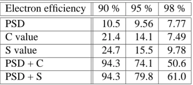
We can identify electrons from pions using calorimeters by utilizing the difference in the lateral shower profile of electromagnetic and hadronic showers. The preshower detector can also be used for electron identification. As the response of the preshower detector is almost independent of the lateral shower spread, a combination of the calorimeters and the preshower detector can improve for electron identification.

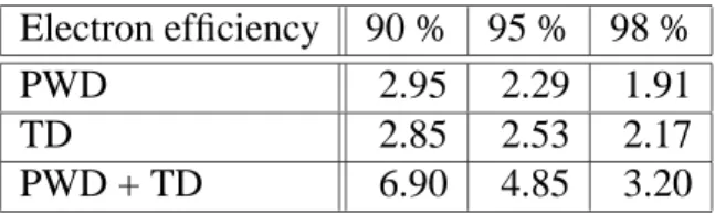
In addition, we may be able to separate electrons and pions by utilizing the difference in the time structure of electromagnetic and hadronic showers.

Electron Identification from Lateral Shower Spread

To characterize the lateral shower spread we defined here two variables . One is the containment value

defined as

¸ 6 ¦]¨

‚ ¨

Vb©

;

9

¦'»

‚ »

V½¼

;

¾

!

:

D%

‹ºs­

:¿ƒ

®DªŸˆ

º « © 9P

^

The suffix

includes the center segment located at the beam position and its eight neighboring ones, while the suffix

includes all test modules and the leakage shower counters. The other variable is the lateral shower spread

defined as

® 6 ¦ ¨¯

2

¨ ‚ ¨

¦ ¨ ‚ ¨

where

is the distance from the beam position determined by drift chambers to the center position of each segment. Fig. 28 shows the distributions of

and

for electrons and pions of momentum 2.5 GeV/c.

In the preshower detector the distribution for pion has a peak which corresponds to the response of a single minimum ionizing particle, while the energy deposits for electrons show broad distributions at much higher region. Fig. 29 shows the pulse height distributions in the preshower detector for electrons and pions of momentum 2.5 GeV/c.

The scatter plots of the preshower detector signal and

or

values are shown in Fig. 30 and Fig. 31, respectively. These figures indicate the electron identification with the test modules in combination with the preshower detector.

We get the electron efficiency and the pion rejection factor as the following expressions, respectively.

‚ 9

!r

‹

ˆÀ

¹¹

© 9

©Áˆ

9P¥

:

‚ÄìÅ

(

Â

‚œÆ

|Ç|

~©

‹

ˆÀr4Y¼Ÿ

9

!©

‹ ˆ ¹ ª 9 ‹ r

:

~ Æ

|È|

 ~ ÃÉÅ

(

Â

‚ÄÆ

|È|

was a number of single-track events selected by DC and

Â

‚ÄÃÉÅ

(

was a number of electron events selected by the calorimeter or PSD, where we used electron data.

 ~ Æ

|Ç|

and

 ~ ìÅ

(

are same definition, where we used pion one. To compare the above analysis by pion rejection factor with fixed electron efficiency, various cuts apply to the data. They are summarized in Table 5.

Although the energy is low, results are good. Especially, the test modules in combination with the preshower detector have good capability to the electron identification. ( At the 98% electron efficiency the pion rejection factor already exceeds 50. )

Electron efficiency 90 % 95 % 98 %

PSD 10.5 9.56 7.77

C value 21.4 14.1 7.49

S value 24.7 15.5 9.78

PSD + C 94.3 74.1 50.6

PSD + S 94.3 79.8 61.0

Table 5: Pion rejection factor for various technique.

Electron Identification from Time Structure

Electromagnetic or hadronic showers have different timing time characteristics. The differences

between electron and pion signals came from the following characteristics.