• 検索結果がありません。

Complex Contact Structures on Nilmanifolds

N/A
N/A
Protected

Academic year: 2021

シェア "Complex Contact Structures on Nilmanifolds"

Copied!
76
0
0

読み込み中.... (全文を見る)

全文

(1)

Complex Contact

Structures on Nilmanifolds

2014

Akira Tanaka

Department of Mathematics and Information Sciences

Tokyo Metropolitan University

(2)
(3)

Contents

Overview 1

I Complex Contact Structures on Nilmanifolds 3

1 Introduction to Part I 5

1.1 Background and Results . . . . 5

2 Similarity Manifolds 9 2.1 Developing Maps . . . . 9

2.2 Similarity Manifolds . . . . 10

2.2.1 Euclidean Similarity Manifolds . . . . 10

2.2.2 Heisenberg Similarity Manifolds . . . . 15

3 Complex Contact Structure on the Nilpotent Group 17 3.1 Definition of Complex Contact Structure . . . . 17

3.2 The Iwasawa Lie Group . . . . 17

3.3 Complex Contact Transformations . . . . 18

3.4 Complex Contact Similarity Geometry . . . . 20

3.5 Proof of the Main Theorem . . . . 22

3.6 Variations . . . . 25

3.6.1 Proof of Theorem 3.6.1 . . . . 26

4 Connected Sum 31 4.1 Connected Sum . . . . 31

5 Contact Structure from Quaternionic Heisenberg Lie Group 33 5.1 Quaternionic Heisenberg Geometry . . . . 33

5.2 Quaternionic Carnot-Carath´ eodory Structure on M . . . . 34

5.3 Complex Contact Bundle on L . . . . 35

(4)

CONTENTS

II Mapping Class Group 37

6 Introduction to Part II 39

6.1 Dehn Twists . . . . 40

6.2 Finite Generating Sets for the Mapping Class Group . . . . 42

7 Torelli Group and Johnson Filtration 47 7.1 The Torelli Group . . . . 47

7.2 Johnson Filtrations . . . . 50

7.3 The Lower Central Series of the Torelli Group . . . . 53

7.4 The Johnson Homomorphism . . . . 54

7.5 The Birman-Craggs Homomorphism . . . . 58

8 Birman Exact Seqence 61 8.1 Forget Maps and Push Maps . . . . 61

8.2 The Birman Exact Sequence for the Johnson filtrations . . . . . 65

(5)

Overview

Part I

The main object of Part I is to study complex contact manifolds. We in- troduce the Iwasawa Lie group L and construct holomorphic group actions on L .

Chapter 1. We explain a background and a history of complex contact manifolds and state our main results.

Chapter 2. We study the notion of developing maps which is an essential tool to prove our main results and collect several previous results on similarity geometry.

Chapter 3. We construct the Iwasawa nilpotent Lie group L . Considering similarity group actions on L , we obtain complex contact similarity manifolds and give a classification on compact complex contact similarity manifolds under a certain assumption.

Chapter 4. Let L /Γ be a complex contact infranilmanifold which is a holomorphic torus bundle over the quaternionic euclidean orbifold. Then we prove that the connected sum of L /Γ with the complex projective space CP 2n+1 admits a complex contact structure.

Chapter 5. We verify L from the viewpoint of geometric structure. The quaternionic Heisenberg Lie group M is known to posses a quateronic Carnot- Carath´ eodory structure (qCC-structure). In fact M occurs as a central group extension 1 R 3 → M −→ H n 1 where R 3 = Im H is the imaginary part of the quaternion field H . Taking a quotient of M by R (= R i), it turns out that the quotient group is the Iwasawa nilpotent group L (= L 2n+1 ) which admits a complex contact structure induced from the qCC-structure on M .

Part II

The main object of Part II is to study the mapping class groups on a surface, the group of isotopy class of the diffeomorphisms on a surface. We study a certain filtration of the mapping class group called the Johnson filtration and give the Johnson filtration version of the Birman exact sequence.

Chapter 6. We introduce some basic results concerning the mapping class

groups and Dehn twists. We show that the Humphrie generator which is an

generator of the mapping class group is obtained from the Lickorish generator.

(6)

CONTENTS

Chapter 7. We recall the Torelli group which is the kernel of the symplectic representation of the mapping class group, and consider the Johnson filtration.

We also give some lemmas to prove the main result of Part II.

Chapter 8. We study homomorphisms from the mapping class group of a subsurface S

of S to the mapping class group of S which is induced by the inclusion of the subsurface S

, S. We introduce a classical tool for studying the mapping class group called the Birman exact sequence, and give the shape of the kernel of this short exact sequence which restricts it to the Johnson filtrations.

Acknowledgment

The author gratefully acknowledges to his advisor Yoshinobu Kamishima for

many helpful advices, encouragements and kindly supports. He also appreciates

the examiners for their cooperation.

(7)

Part I

Complex Contact

Structures on Nilmanifolds

(8)
(9)

Chapter 1

Introduction to Part I

1.1 Background and Results

The notion of a complex contact manifold was first introduced by Kobayashi[32]

in 1959 as a complex analogue of (real) contact manifold.

There are constructions of three different types of complex contact struc- ture. Given a 4n-dimensional quaternionic K¨ ahler manifold M which locally has a quaternion structure {I , J , K} , we can obtain the twistor space Z locally described as

Z = { x I + y J + z K | x 2 + y 2 + z 2 = 1 } ⊂ End(T M ).

This is the total space of the S 2 bundle S 2 Z M.

Salamon[52] proved that the twistor space of a quaternionic K¨ ahler manifold of nonzero scalar curvature admits a complex contact structure.

Similarly, a quaternionic K¨ ahler manifold M 4n of positive (resp. nega- tive) scalar curvature induces a Sasakian 3-structure (resp. pseudo-Sasakian 3-structure) on the total space P 4n+3 of the principal bundle: S 3 P M . Dividing by the free action induced by a Reeb vector field, we obtain the fol- lowing diagram.

S 3 −−−−→ P −−−−→ M

/S

1

 

y /S

1

  y S 2 −−−−→ P/S 1 −−−−→ M

The total space P/S 1 of the quotient bundle S 2 P/S 1 N admits a complex contact structure. (See Ishihara & Konishi[22]; Moroianu & Semmelmann[46];

Tanno[53].) However, these constructions cannot produce complex contact man-

ifolds for quaternionic K¨ ahler manifolds of vanishing scalar curvature.

(10)

CHAPTER 1. INTRODUCTION TO PART I

On the other hand, if N 4n is a complex symplectic manifold with a com- plex symplectic form Ω = Ω 1 + iΩ 2 such that [Ω i ] H 2 (N; Z ) is an integral class (i = 1, 2), then the complex Boothby-Wang fibration induces a compact complex contact manifold M which has a connection bundle: T 2 M N (cf. Foreman[16]; Blair[9]). If N 4n happens to be a quaternionic K¨ ahler man- ifold with vanishing scalar curvature, then we have a new example of compact complex manifold. In fact, Foreman[16] shows that a complex nilmanifold M which is the total space of a principal torus bundle over a complex torus T

C

2n admits a complex contact structure. The universal covering ˜ M is endowed with a complex nilpotent Lie group structure which is called the generalized complex Heisenberg group in Foreman[16].

In Part I, we study complex contact transformation groups by taking into account this specific nilpotent Lie group.

In Chapter 3, we give the definition of a complex contact manifold and con- struct complex contact similarity manifolds. We are mainly interested in con- structing examples of compact complex contact manifolds which are not known previously. Let Sim( L ) be the group of complex contact similarity transforma- tions. It is defined to be the semidirect product L⋊ (Sp(n) ·C

) ( C

= S 1 ×R + ).

The pair (Sim( L ), L ) is said to be complex contact similarity geometry. A man- ifold M locally modelled on this geometry is called a complex contact similarity manifold. Denote by Aut cc (M ) the group of complex contact transformations of M .

A similarity manifold is defined in Fried[17]. We define this object in Chapter 2.

Theorem 1.1.1 (Fried[17]). Let M be a closed similarity manifold. Then M is finitely covered by either a flat torus or a Hopf manifold.

On the other hand, Miner proved the following CR analogue of the theorem by Fried.

Theorem 1.1.2 (Miner[41]). Let M be a compact spherical CR-manifold with amenable holonomy. Then M is finitely covered by S 2n+1 , S 1 × S 2n

2 or a compact quotient of the Heisenberg group H where Γ is lattice in H .

He showed that, if M is complete, then M is covered by S 2n+1 ; otherwise M has the structure of a Heisenberg similarity manifold.

We prove the following characterization of compact complex contact simi- larity manifolds in Chapter 3. This theorem can be thought of as a quaternion version of the above theorems.

Theorem A. Let M be a compact complex contact similarity manifold of com-

plex dimension 2n + 1. If S 1 Aut cc (M ) acts on M without fixed points, then

M is holomorphically isomorphic to a complex contact infranilmanifold L or

a complex contact infra-Hopf manifold L − { 0 } which is finitely covered by a

Hopf manifold S 4n+1 × S 1 . Here Γ is a discrete cocompact virtually nilpotent

subgroup in L ⋊ (Sp(n) · S 1 ) or isomorphic to the product of a cyclic group with

an infinite cyclic subgroup Z p × Z + of Sp(n) · S 1 × R + .

(11)

1.1. BACKGROUND AND RESULTS Proposition B. The following hypothesis (i) or (ii) yields the same conclusion of Theorem A.

(i) The holonomy group is virtually nilpotent.

(ii) The holonomy group is discrete.

In Chapter 4, we can perform a connected sum of our complex contact infranilmanifolds L /Γ (Γ E( L )).

Theorem C. The connected sum CP 2n+1 # L admits a complex contact struc- ture.

By iteration of this procedure there exists a complex contact structure on the connected sum of a finite number of complex contact similarity manifolds and CP 2n+1 ’s.

Corollary D. Any connected sum M 1 # · · · #M k #ℓ CP 2n+1 admits a complex contact structure for a finite number of complex contact similarity manifolds M 1 , . . . , M k and ℓ-copies of CP 2n+1 .

These examples are different from those admitting S 2 (resp. T 2 )-fibrations.

In Chapter 5, we verify L from the viewpoint of geometric structure. In fact the sphere S 4n+3 admits a canonical quaternionic CR-structure. The sphere S 4n+3 with one point removed is isomorphic to the 4n+3-dimensional quater- nionic Heisenberg Lie group M as a quaternionic CR-structure. M has a central group extension : 1 R 3 → M −→ p H n 1 where R 3 = Im H is the imaginary part of the quaternion field H . Taking a quotient of M by R (= R i), we ob- tain a complex nilpotent Lie group L (= L 2n+1 ) which supports a holomorphic principal bundle C → L −→ p C 2n . The canonical quaternionic CR-structure on S 4n+3 restricts a Carnot-Carath´ eodory structure B to M . Using this bundle B, a left invariant complex contact structure on L is obtained (cf. Alekseevsky

& Kamishima[1]; Kamishima[29]).

Results of Part I are from Kamishima & Tanaka[30].

(12)
(13)

Chapter 2

Similarity Manifolds

2.1 Developing Maps

Definition 2.1.1. Let X be a connected smooth manifold, and suppose a group G acts on X via diffeomorphisms transitively. Then a manifold M satisfying following conditions is called a (G, X)-manifold.

1. There exists an open cover { U α } α

Λ of M and a family of maps ϕ α : U α V α

each of which is a diffeomorphism onto its image V α := ϕ α (U α ) in X.

2. If U α U β ̸ = , then there exists an element g G s.t.

g = ϕ α ϕ

β 1 , on V α V β .

The second condition of Definition 2.1.1 says that, if we think of G as dif- feomorphisms of X, each transition functions

γ αβ = ϕ α ϕ

β 1 : V α V β V α V β

is the restriction of an element of G to V α V β .

Example. If G is the group of isometries of Euclidean space E n , then (G, E n )- manifold is called a Euclidean, or flat, manifold. If G is the group of affine transformations of R n , then (G, R n )-manifold is called an affine manifold.

Take a (G, X)-manifold M . Let (U α , ϕ α ) and (U β , ϕ β ) be two charts of M

and suppose x U α U β . By the definition of (G, X)-manifold, on U α U β ,

ϕ α and ϕ β differ by γ αβ . Thus composing γ αβ to ϕ β , we obtain ϕ α extended to

U α U β . Fix a family of charts of M and consider a path α(t), t [0, 1] on M s.t

α(0) U α . Then we go along α and modify the function at each intersection of

charts. And we successively extend ϕ α . But in general we can not extend ϕ α to

(14)

CHAPTER 2. SIMILARITY MANIFOLDS

whole M in this way, since it is necessary to coincide ϕ α and modified function when α(1) is again in U α . One of sufficient conditions to extend to M is that M is simply connected. So we consider the universal covering of π : ˜ M M and define a map on it as follows. First we think of ˜ M as the space of homotopy classes of paths in M which start at the fixed basepoint in U 0 . We take a path α representing a point [α] M ˜ s.t. α(1) = π([α]). Then we extend ϕ 0 along α and obtain

ψ = γ 01 γ 12 · · · γ n

1,n ϕ n .

It can be shown that ψ depends on only the first choice of charts and homotopy class of α. So we set ϕ [α] = ψ.

Definition 2.1.2 (see Thurston[55]). Fix a basepoint and initial chart ϕ α . The developing map of a (G, X)-manifold M is the map

dev : ˜ M X

defined as dev = ϕ [α] π in a neighborhood of [α] M ˜ .

Note that other choices of the basepoint and the initial chart cause the difference by composition in the range with an element of G.

We use dev to give the classification of complex contact similarity manifolds.

For this purpose, we state the following proposition.

Proposition 2.1.3 (see Cheeger & Ebin[11]). If f : (M, g M ) (N, g N ) is a local isometry and M is complete, then f : M N is a covering map.

By this proposition, if we find a metric on the manifold which is domain of dev s.t. dev becomes a local isometry, then dev becomes a covering map.

2.2 Similarity Manifolds

2.2.1 Euclidean Similarity Manifolds

A Euclidean similarity manifold M is an affine manifold whose holonomy group lies in the group Sim( E n ) := R n × (O(n) × R + ) of Euclidean similarity trans- formations of E n . A developing map determines similarities ρ(g) Sim( E n ), where g π 1 (M ), with the property that

ρ(g) dev = dev g : ˜ M E . So we have

ρ : π 1 (M ) Sim( E n ).

We call the pair (ρ, dev) developing pair. If ρ(π 1 (M )) fixes a single point, then we say the similarity manifold is radiant. Fried[17] showed the following theorem.

Theorem 2.2.1 (Fried[17]). A compact incomplete Euclidean similarity mani-

fold is radiant.

(15)

2.2. SIMILARITY MANIFOLDS Choosing the fixed point as origin, radiant similarity structures are based on the group of linear similarities Sim 0 ( E n ) := Sim( E n ) GL(n, R ). Fried also showed geodesically complete similarity manifolds are Euclidean. So Theorem 2.2.1 shows that the structure group of a similarity manifold is always reduced to Sim 0 ( E n ) or the Euclidean group Euc( E n ). Thus we have Theorem 1.1.1. In this section, we explain Theorem 2.2.1 along Miner[41].

First, we need some preparation. Fix dev : ˜ M E n . This defines the pull- back metric dev

g

E

on ˜ M and scale factors α : Sim( E ) R + by | gv | = α(g) | v | for g Sim( E ), v E .

The exponential map for M is the affine map exp : E → M defined on an open subset E ⊂ T M s.t. for each v ∈ E the path γ(t) = exp(tv) for 0 t 1 is the affinely parametrized geodesic on M with velocity vector v at t = 0. For each m M we define its exponential domain E m to be E ∩ T m M .

We define

Exp : T E (= E ) E

to be the exponential map for T E and the following diagram is commutative.

T M ˜ −−−−→ d dev T E

exp

 

y   y Exp M ˜ −−−−→

dev E

Since M is locally modelled on E , we have D : T M ˜ E s.t. D | T

m˜

M ˜ = Exp d dev.

Proposition 2.2.2. Let M be an affine manifold, g be an element in the group of affine transformations Aff( E ) and U be a convex subset of dev( ˜ M ). If U ⊂ g(dev( ˜ M )) and g( V ) ⊂ U , then (D | T

m˜

M ˜ )

1 ( V ) ⊂ E m ˜ .

By the assumption that M is an incomplete similarity manifold, we define a function R : ˜ M R + by R( ˜ m) to be the radius of the largest open ball in T m ˜ M ˜ on which exp is defined. More precisely,

R( ˜ m) = sup { r |E m contains a ball of radius r with respect to dev

g

E

} .

We denote the ball as D m ˜ .

(16)

CHAPTER 2. SIMILARITY MANIFOLDS

Fig. 2.1

Fig. 2.1 shows that R( ˜ m) R(˜ n) dist( ˜ m, ˜ n). Thus we have the following.

Lemma 2.2.3. R satisfies | R(x) R(Y ) | ≤ dist(x, y). Namely R is Lipschitz.

So we have the following lemma.

Lemma 2.2.4. Let g π 1 (M ) and ρ(g) is a similarity transformation. Then D g ( ˜ m) = dg(D m ˜ ) and R(g m) = ˜ α(ρ(g))R( ˜ m).

From this lemma,

g M ˜ ( ˜ m) := dev

g

E

( ˜ m)/R 2 (x)

defines a Riemannian metric g M ˜ on ˜ M which is invariant under π 1 (M ). This metric is conformal to the flat metric dev

g

E

, and D m ˜ is the unit disk with respect to this metric. Since g M ˜ is π 1 (M )-invariant, there exists a Riemannian metric g M on M s.t.

π

g M = f M ˜ . Hence we have the following.

Proposition 2.2.5. Let M be an incomplete similarity manifold. Then there exists a unique continuous conformal Riemannian metric for which the unit ball in T m M is the maximum ball contained in the exponential domain E m for each m M

For fixed ˜ m M ˜ , let v 0 ∂D m ˜ be a vector s.t. the affine geodesic ˜ γ = exp(tv 0 ) is defined for 0 t < 1 but not for t = 1. By the definition, ˜ γ(t) does not converge as t 1 although it does in the developing image, dev(˜ γ(t)) Exp(d dev(v 0 )).

Since M is compact, γ(t) := π ˜ γ has a point of accumulation y M and there exists an ϵ-ball B centers at y which γ(t) must exits every time it enters.

Pick a sequence of times;

0 < t 0 < t 1 < · · · < t n < · · ·

(17)

2.2. SIMILARITY MANIFOLDS with t n 1 s.t. γ(t i ) is in B but γ([t i , t i+1 ]) is not in B. Namely at each interval, γ(t) exits B. For each i, let η i be the radial geodesic from y to γ(t i ) contained in B. Then we can define elements g ij π 1 (M, y) as follows. Starting at y and we go along η i , γ | [t

i

,t

j

] , and η

j 1 . (See Fig. 2.2.)

Fig. 2.2

Thus we obtain a family { g ij } in π 1 (M ). Now we consider the actions of these elements in the developing image.

Let g be an element of Sim( L ), then the action is written as g(x) = c + αA(x c)

where c R n , α R + and A O(n). If g(X ) = Y , then c can be written as c = (I αA)

1 (Y αA(X )).

When X = dev(˜ γ(t i )), Y = dev(˜ γ(t j )), A = I and α = (1 t j )/(1 t i ), it can be shown that for j >> i >> 0, the above equation reduces to c = v 0 . On the other hand, since O(n) is compact, the matrices { A ij } must accumulate. And ρ(g jk ) ρ(g ij ) = ρ(g ik ) implies that A jk A ij = A ik . Hence | A ij I | < ϵ for infinitely many { i, j } . So we have the following lemma.

Lemma 2.2.6. For sufficiently large i and j, we can choose ρ(g ij ) to be a similarity centered arbitrarily close to v 0 with almost no rotation.

From Lemma 2.2.4, there exists a half space neighborhood of the origin in each tangent space on which the exponential map is defined. Let

H m ˜ = { w ˜ T m ˜ M ˜ | µ( ˜ ˜ w, v ˜ 0 ) 1 } .

(18)

CHAPTER 2. SIMILARITY MANIFOLDS Decompose the boundary of H m ˜ into visible set

J m ˜ = { w ˜ ∂H m ˜ | exp m ˜ ( ˜ w) is defined } and invisible set

I m ˜ = { w ˜ ∂H m ˜ | exp m ˜ ( ˜ w) is undefined } .

As mentioned above, we can choose ρ(g ij ) close to a homothety centered at v 0 . The set D ij := ρ(g ij )

1 (ρ(g ij )(D(D m ˜ )) D(D m ˜ )) satisfies the hypotheses of Proposition 2.2.2. D

1 (D ij ) can be made to approximate D m ˜ arbitrarily well. Thus for sufficiently large i, j, k, D(H m ˜ ) is in ρ(g ij )

k (D ij ) and apply Proposition 2.2.2, we have H m ˜ ⊂ E m ˜ .

Lemma 2.2.7. I m ˜ is an affine subspace of ∂H m ˜ .

Proof. Suppose there exists an n J m ˜ , and let ˜ n = exp n. Then ˜ n has a neighborhood H n ˜ on which exp ˜ n is defined. We claim that D(v 0 ) is in ∂(D(H ˜ n )).

If D(v 0 ) / ∂(D(H n ˜ )), consider the action of ρ(g ij )

1 . This takes D(H n ˜ ) into itself, and so by Proposition 2.2.2, exp n ˜ is defined on ρ(g ij )(H n ˜ ). But the

∂(D(H n ˜ )) is contained in ρ(g ij )(H n ˜ ) which is contradiction.

For any point in I m ˜ , there exists an associated family of contraction { ρ(γ ij ) } and we can use the same argument as above. Thus we have

I m ˜ ∂(D(H m ˜ )) ∂(D(H n ˜ ))

This is an affine subspace of dimension dim(∂H m ˜ ) 1. If there are no visible points in this intersection, it is in fact I m ˜ and the lemma is proved. Otherwise, repeat the process to show I m ˜ is contained in an affine subspace of dim(∂H m ˜ ) 2.

Since this procedure must terminate, the lemma is proved.

It can be shown that I := D(I m ˜ ) is locally constant, so I / dev( ˜ M ). Define the vector field ˜ X on ˜ M by specifying its value at each point to be the shortest vector for which exp is undefined. By Lemma2.2.4, this vector field is π 1 (M ) invariant and thus defines a vector field X on M . X is seen to correspond to the vector field Y on E d which assigns to x E d the vector Y (x) from x to I which is perpendicular to I. Let ˜ ω be the standard volume form on ˜ M and R(p)

1 ω ˜ is π 1 (M ) invariant. Thus we can obtain ω which is a volume form on M . Computation shows div ω (X ) = dim(I). By Green’s theorem, we have dim(I) = 0 and so X is a radiant vector field. This proves Theorem 2.2.1.

Take a closed connected euclidean similarity manifold M , As a consequence of Theorem 2.2.1, Fried gave the following classification.

Theorem 2.2.8 (Fried[17]). If M is complete, then M is Euclidean. Otherwise

M is radiant.

(19)

2.2. SIMILARITY MANIFOLDS

2.2.2 Heisenberg Similarity Manifolds

Let H be the Lie group C n × R with group law:

(ζ, v)(ξ, w) = (ζ + ξ, v + w + Im ζ, ξ ).

Here ζ, ξ = ∑ n

i=1 ζ i ξ ¯ i . And α · A U(n) × R + acts on H as:

α · A(ζ, v) = (αAζ, α 2 v),

where α R + and A U (n). We denote the Heisenberg similarity group H × (U(n) × R + ) as Sim( H ).

CR-structure is a real codimension 1 subbundle of the tangent bundle with an integrable complex structure on it. The canonical CR-structure on ∂B n C n is given at each point by taking the maximal complex subspace J (T x ∂B n ) T x ∂B n of T ∂B n . Since we can think of the boundary of complex hyperbolic space as the one point compactification of the Heisenberg group, we can think of H as a subset of ∂B n . So H inherits this CR-structure.

A (real) contact structure on a 2n 1-dimensional manifold X is a 1-form ω s.t. ω (dω) n

1 ̸ = 0. Let ω be a contact form on ∂B n and set E = { x T (∂B n ) | ω(x) = 0 } . If E is the subbundle giving the CR-structure on ∂B n , then we say ω is a calibration for the CR-structure. We call Ker ω | x the contact plane at x which defines a notion of horizontal at a point. We say a vector field X is CR-horizontal if ω(X) = 0. In Heisenberg coordinates, the contact plane at the origin corresponds to { (ζ, v) ∈ H | v = 0 } .

We explain the following generalization of Theorem 2.2.1.

Theorem 2.2.9 (Miner[41]). A compact incomplete Heisenberg similarity man- ifold is radiant.

We can pull back a metric d

H

on H to T m ˜ M ˜ via the map D and de- note it as d

H

too. Define R

H

( ˜ m) to be the radius of the largest Heisen- berg ball D m ˜ T m ˜ M ˜ centered at the origin on which the exponential map is defined. And let α

H

: Sim( H ) R + be a homomorphism defined by

| g(ζ, v) |

H

= α

H

(g) | (ζ, v) |

H

for g Sim( H ). Then we can check that Lemma 2.2.3, Lemma 2.2.4 and Proposition 2.2.6 still hold in the Heisenberg case.

Lemma 2.2.10. R

H

is Lipschitz with respect to d

H

. D g ( ˜ m) = dg(D m ˜ ) and R

H

(g m) = ˜ α

H

(ρ(g))R( ˜ m) for g Aut( ˜ M ).

Fix a point ˜ m M ˜ and (ζ 0 , v 0 ) ∂D m ˜ s.t. ¯ γ(t) = exp m ˜ (tζ 0 , tv 0 ) is in- complete. In the same way that we did in the Euclidean case, we can choose a family { g ij } in π 1 (M ) associated to any incomplete geodesic which has a point of accumulation in M . Then we have the following lemma.

Lemma 2.2.11. For sufficiently large i and j, we can choose ρ(g ij ) to be a

Heisenberg similarity centered arbitrarily close to D(ζ 0 , v 0 ) with almost no rota-

tion.

(20)

CHAPTER 2. SIMILARITY MANIFOLDS

By this lemma and Proposition 2.2.2, we can expand the region D m ˜ T m ˜ M ˜ to a half space H m ˜ on which exp is defined. Recall that ∂H m ˜ is divided into sets J m ˜ and I m ˜ of visible and invisible points, and I m ˜ is the intersection of planes ∂H n ˜ as ˜ n ranges over various points in J m ˜ . It follows that I m ˜ is an affine subspace of ∂H m ˜ . Let I be the constant image dev(I m ˜ ) as ˜ m ranges over ˜ M . Miner showed the following lemma.

Lemma 2.2.12 (Miner[41]). I is CR-horizontal.

So suppose I is CR-horizontal and assume the developing map was chosen so that I passes through the origin without loss of generality. It can be checked that the maximal CR-horizontal subspace passing through the origin in Heisenberg space is conjugate to the n dimensional subspace E of real points of C n thinking of H as C n × R .

Since ρ(π 1 (M )) must stabilize I, ρ(π 1 (M )) lies in the subgroup of Sim( H ) which stabilizes the real points. The subgroup of U(n) which stabilizes the real points is isomorphic to O(n). The Heisenberg translations stabilizing the real points are those of the form (ζ, 0) where ζ is a real vector. The Heisenberg dilation stabilizing the real points are those centers lie in the set of real points.

Thus the action of Stab( E , Sim( H )) agrees with the action of Sim( R 2n

1 ) on E . Define

h(x) = x | x | and

ϕ(z, v) = (z, h

1 (v + x · y))

where x R and z = x+iy. Then Stab( E , Sim( H )) is conjugate to Stab( E , R 2n

1 ) by ϕ. Let H(ζ, v) be the Heisenberg translation by (ζ, v), then for a real vector r, we have

ϕ H (r, 0) ϕ

1 (z, v) = (z + r, v).

Similarly, let D α be the Heisenberg dilation by α centered at the origin, then ϕ D α ϕ

1 (z, v) = (αz, αv).

If A U(n), then we have

ϕ A ϕ

1 (ζ, v) = (Aζ, v).

Thus we have

ϕ Stab( E ) ϕ

1 Sim( R 2n

1 ).

So ϕ dev gives M a Euclidean similarity structure:

M ˜ −−−−→ H dev −−−−→ ϕ R 2n+1

g

 

y   y ρ(g)   y ϕ

ρ(g)

ϕ

−1

M ˜ −−−−→ H dev −−−−→ ϕ R 2n+1

Since ϕ(I) = I, this structure is also incomplete. By applying Theorem 2.2.8,

we have Theorem 2.2.9 and as a consequence of Theorem 2.2.9, Theorem 1.1.2

follows.

(21)

Chapter 3

Complex Contact Structure on the Nilpotent Group

3.1 Definition of Complex Contact Structure

Recall that a complex contact structure on a complex manifold M in complex dimension 2n + 1 is a collection of local forms { U α , ω α } α

Λ which satisfies that (1)

α

Λ U α = M . (2) Each ω α is a holomorphic 1-form defined on U α . Then ω α (dω α ) n ̸ = 0 on U α . (3) If U α U β ̸ = , then there exists a nonzero holo- morphic function f αβ on U α U β such that f αβ · ω α = ω β . Unlike contact structures on orientable smooth manifolds, it does not always exist a holomor- phic 1-form globally defined on M . Note that if the first Chern class c 1 (M ) vanishes, then there is a global existence of a complex contact form ω on M . (See Kobayashi[32]; Lebrun[35])

Let h : M M be a biholomorphism. Suppose that h(U α ) U β ̸ = for some α, β Λ. If there exists a holomorphic function f αβ on an open subset in U α such that h

ω β = f αβ ω α , then we call h a complex contact transformation of M . Denote Aut cc (M ) the group of complex contact transformations. It is not necessarily a finite dimensional complex Lie group.

3.2 The Iwasawa Lie Group

Let L 2n+1 be the product C 2n+1 = C × C 2n with group law (n 1):

(x, z) · (y, w) = (x + y +

n i=1

z 2i

1 w 2i z 2i w 2i

1 , z + w)

where z = (z 1 , . . . , z 2n ), w = (w 1 , . . . , w 2n ).

(22)

CHAPTER 3. COMPLEX CONTACT STRUCTURE ON THE NILPOTENT GROUP

Put L = L 2n+1 . It is easy to see that [(x, z), (y, w)] = (2

n i=1

z 2i

1 w 2i z 2i w 2i

1 , 0) so [ L , L ] = ( C , (0, . . . , 0)) = C is the center of L . Thus there is a central group extension: 1 C → L 2n+1 −→ C 2n 1. It is easy to check that L 3 is isomorphic to the Iwasawa group consisting of 3 × 3-upper triangular unipotent complex matrices by the following correspondence.

(c, (a, b)) 7→

 1 a ab+c 2

0 1 b

0 0 1

Definition 3.2.1. A complex 2n + 1-dimensional complex nilpotent Lie group L 2n+1 is said to be the Iwasawa Lie group.

See Foreman[16], pp.193-195 for more general construction of this kind of Lie group.

Now we construct a complex contact structure on L 2n+1 . Choose a coordi- nate (z 0 , z 1 , . . . , z 2n ) ∈ L 2n+1 , we define a complex 1-form η:

η =dz 0 (

n i=1

z 2i

1 · dz 2i z 2i · dz 2i

1 )

= dz 0 (z 1 , . . . , z 2n ) J n

  dz 1

.. . dz 2n

 

where J n =

  J

. . . J

  with J =

( 0 1

1 0 )

.

Since η (dη) n is a non-vanishing form 2n( 2) n dz 0 ∧ · · · ∧ dz 2n on L 2n+1 , η is a complex contact structure on L 2n+1 by Definition 2.1.1.

3.3 Complex Contact Transformations

Let hol( L 2n+1 ) be the group of biholomorphic transformations of L = L 2n+1 . The group of complex contact transformations on L with respect to η is denoted by

hol( L , η) = { f hol( L ) | f

η = τ · η } where τ is a holomorphic function on L .

Let Sp(n, C ) = { A M (2n, C ) | t AJ n A = J n } be the complex symplectic group. As Sp(n, C ) C

= 1 } , denote Sp(n, C ) · C

= Sp(n, C ) × C

/ 1 } . Put

A( L ) = L ⋊ (Sp(n, C ) · C

)

(23)

3.3. COMPLEX CONTACT TRANSFORMATIONS which forms a group as follows; write elements λ · A, µ · B Sp(n, C ) · C

for A, B Sp(n, C ), λ, µ C

. Let (a, w), (b, z) ∈ L . Define

( (a, w), λ · A )

· (

(b, z), µ · B )

= (

(a + λ 2 b + t w J n (λAz), w + λAz), λµ · AB ) .

Here t w J n (λAz) =

n i=1

w 2i

1 · (λAz) 2i w 2i · (λAz) 2i

1 as before.

Let (

(a, w), λ · A )

A( L ), (z 0 , z) ∈ L . A( L ) acts on L as ( (a, w), λ · A )

· (z 0 , z) = (a, w) ·2 z 0 , λAz)

= (a + λ 2 z 0 + t w J n (λAz), w + λAz). (3.1) If h = ((b, w), µ · B) A( L ) is an element, then it is easy to see that

h

η = µ 2 · η. (3.2)

Thus A( L ) preserves the complex contact structure on L defined by η.

Let Aff( C 2n+1 ) = C 2n+1 ⋊ GL(2n + 1, C ) be the complex affine group which is a subgroup of hol( L ) since L 2n+1 = C n+1 (biholomorphically). We assign to each (

(a, w), λ · A )

A( L ) an element ([ a

w ]

,

( λ 2 λ t w J n A

0 λA

)) Aff( C 2n+1 ).

Then the action (3.1) of (

(a, w), λ · A )

on L coincides with the above affine transformation of C 2n+1 . Moreover, it is easy to check that this correspondence is an injective homomorphism:

A( L ) Aff( C 2n+1 ). (3.3)

As a consequence it follows

A( L ) hol( L , η).

Let M be a smooth manifold. Suppose that there exists a maximal collec- tion of charts { (U α , φ α ) } α

Λ whose coordinate changes belong to A( L ). More precisely, M =

α

Λ U α , φ α : U α → L is a diffeomorphism onto its image.

If U α U β ̸ = , then there exists a unique element g αβ A( L ) such that g αβ = φ β · φ

α 1 on φ α (U α U β ). We say that M is locally modelled on (A( L ), L ).

(Compare Kulkarni[34].)

Here is a sufficient condition for the existence on complex contact structure.

Proposition 3.3.1. If a (4n + 2)-dimensional smooth manifold M is locally

modelled on (A( L ), L ), then M is a complex contact manifold. Moreover, M is

also a complex affinely flat manifold.

(24)

CHAPTER 3. COMPLEX CONTACT STRUCTURE ON THE NILPOTENT GROUP

Proof. First of all, we define a complex structure on M . Let J 0 be the standard complex structure on L = C 2n+1 . Define a complex structure J α on U α by setting φ α

J α = J 0 φ α

on U α for each α Λ. When g αβ A( L ), note that g αβ

J 0 = J 0 g αβ

from (3.3). On U α U β , a calculation shows that φ β

J α = g αβ

φ α

J α = J 0 φ β

. Since φ β

J β = J 0 φ β

by the definition, it follows J α = J β

on U α U β . This defines a complex structure J on M . In particular, each φ α : (U α , J) ( L , J 0 ) (= C 2n+1 ) is a holomorphic embedding. Let η be the holomorphic 1-form on L as before. Define a family of local holomorphic 1-forms { ω α , U α } α

Λ by

ω α = φ

α η on U α .

If U α U β ̸ = , then there exists a unique element g αβ A( L ) such that g αβ = φ β · φ

α 1 . From (3.2), g αβ

η = µ 2 αβ · η for some µ αβ C

. It follows ω β = µ 2 αβ · ω α . Thus the family { ω α , U α } α

Λ is a complex contact structure on (M, J).

Apart from the complex contact structure, since A( L ) Aff( C 2n+1 ) from (3.3), M is also modelled on (Aff( C 2n+1 ), C 2n+1 ) where L = C 2n+1 . M is a complex affinely flat manifold.

Remark 3.3.2.

1. When a subgroup Γ A( L ) acts properly discontinuously and freely on a domainof L with compact quotient, we obtain a compact complex contact manifold Ω/Γ by this proposition. In fact let p : Ω Ω/Γ be a covering holomorphic projection. Take a set of evenly covered neighbor- hoods { U α } α

Λ of Ω/Γ. Choose a family of open subsets U ˜ α such that p α = p

|

U ˜

α

: ˜ U α U α is a biholomorphism. Put ω α = (p

α 1 )

η. Then the family { U α , ω α } α

Λ is a complex contact structure on Ω/Γ.

2. When Ω = L , L is said to be a compact complete affinely flat manifold.

Concerning the Auslandr-Milnor conjecture, we do not know whether the fundamental group Γ is virtually polycyclic.

When M is a complex manifold, we assume that the complex structure on M coincides with the one constructed in Proposition 3.3.1.

3.4 Complex Contact Similarity Geometry

It is in general difficult to find such a properly discontinuous group Γ as in Re- mark 3.3.2. Sp(n, C ) contains a maximal compact symplectic subgroup Sp(n) = { A U(2n) | t AJ n A = J n } where Sp(n, C ) = Sp(n) × R n(2n+1) .

Definition 3.4.1. Put Sim( L ) = L ⋊ (Sp(n) ·C

) A( L ). The pair (Sim( L ), L ) is called complex contact similarity geometry. If a manifold M is locally mod- elled on this geometry, M is said to be a complex contact similarity manifold.

The euclidean subgroup of Sim( L ) is defined to be E( L ) = L ⋊ (Sp(n) · S 1 ).

(25)

3.4. COMPLEX CONTACT SIMILARITY GEOMETRY For example, choose c C

with | c | ̸ = 1 and A Sp(n). Put r = (

(0, 0), c · A )

Sim( L ). Let Z + be an infinite cyclic group generated by r. Then it is easy to see that Z + acts freely and properly discontinuously on the complement L−{ 0 } . Here 0 = (0, 0) ∈ L 2n+1 = L . The quotient L−{ 0 } / Z + is diffeomorphic to S 1 × S 4n+1 . By Proposition 3.3.1 (1 of Remark 3.3.2), S 1 × S 4n+1 is a complex contact similarity manifold.

Let H n be the 4n-dimensional quaternionic vector space. The quaternionic similarity group Sim( H n ) = H n ⋊ ((Sp(n) · Sp(1)) × R + ) (resp. quaternionic euclidean group E( H n ) = H n ⋊ (Sp(n) · Sp(1))) has a special subgroup Sim( d H n ) = H n ⋊ ((Sp(n) · S 1 ) × R + ) (resp. E( b H n ) = H n ⋊ (Sp(n) · S 1 )). When we identify H n with the complex vector space C 2n by the correspondence (a + bj) 7→a, b), Sim( d H n ) is canonically isomorphic to the complex similarity subgroup C 2n ⋊ (Sp(n) · C

) where C

= S 1 × R + . Then there are commutative exact sequences:

1 −−−−→ C −−−−→ Sim( L ) −−−−→

p

Sim( d H n ) −−−−→ 1

||

1 −−−−→ C −−−−→ E( L ) −−−−→

p

E( b H n ) −−−−→ 1.

Choosing a torsionfree discrete cocompact subgroup Γ from E( L ), we obtain an infranilmanifold L /Γ of complex dimension 2n + 1. In particular, Γ ∩ L is discrete uniform in L by the Auslander-Bieberbach theorem. As C is the central subgroup of L , Γ C is discrete uniform in C and so ∆ = p(Γ) is a discrete uniform subgroup in E( b H n ). We obtain a Seifert singular fibration over a quaternionic euclidean orbifold H n /∆: T

C

1 → L −→ H n /∆. By 1 of Remark 3.3.2, L /Γ is a complex contact manifold.

Remark 3.4.2. When we take a finite index nilpotent subgroup Γ

of Γ admit- ting a central extension : 1 Z 2 Γ

−→ Z 4n 1, a nilmanifold L

admits a holomorphic principal T

C

1 -bundle over a complex torus T

C

2n = H n / Z 4n . This holomorphic example is a special case of Foreman’s T 2 - connection bundle over T

C

2n (Foreman[16]).

We give rise to a classification of compact complex contact similarity man-

ifolds under the existence of S 1 -actions. (Compare Fried[17]; Miner[41] for the

related results of similarity manifolds.) Recall that Aut cc (M ) is the group of

complex contact transformations defined in section 3.1.

(26)

CHAPTER 3. COMPLEX CONTACT STRUCTURE ON THE NILPOTENT GROUP

Theorem 3.4.3. Let M be a compact complex contact similarity manifold of complex dimension 2n + 1. If S 1 Aut cc (M ) acts on M without fixed points, then M is holomorphically isomorphic to a complex contact infranilmanifold L or a complex contact infra-Hopf manifold L − { 0 } which is finitely covered by a Hopf manifold S 4n+1 × S 1 . Here Γ is a discrete cocompact virtually nilpotent subgroup in L ⋊ (Sp(n) · S 1 ) or isomorphic to the product of a cyclic group with an infinite cyclic subgroup Z p × Z + of Sp(n) · S 1 × R + .

3.5 Proof of the Main Theorem

Let J be a complex structure on M . Given a collection of charts { U α , φ α , J α } on M with J α = J

|

U

α

such that φ α : (U α , J α ) ( L , J 0 ) is a holomorphic diffeomorphism onto its image. Recall that the monodromy argument shows that there is a developing pair:

(ρ, dev) : (Aut cc ( ˜ M ), M ˜ ) (Sim( L ), L )

where ˜ M is the universal covering and ˜ J is a lift of J to ˜ M , and π = π 1 (M ) Aut cc ( ˜ M ). Let J be a complex structure on ˜ M . Then dev is a holomorphic immersion dev

J = J 0 dev

and ρ : Aut cc ( ˜ M ) Sim( L ) is a holonomony homomorphism. Put Γ = ρ(π). Let ˜ S 1 be a lift of S 1 to ˜ M so that ρ( ˜ S 1 ) Sim( L ).

Case 1. If Γ E( L ), then there is a E( L )-invariant Riemannian metric on L . As M is compact, the pullback metric on ˜ M by dev is (geodesically) complete, dev : ˜ M → L is an isometry. As dev becomes a complex contact diffemorphism, M is holomorphically isomorphic to a complex contact infranilmanifold L /Γ.

Case 2. Suppose that some ρ(γ) has a nontrivial summand in R + ≤ L⋊ (Sp(n) · S 1 ×R + ) = Sim( L ). In view of the affine representation ρ(γ) = (p, P ) where P = ( λ 2 λ t w J n A

0 λA

)

from (3.3), we note | λ | ̸ = 1, i.e. P has no eigenvalue 1. Then there exists an element z 0 ∈ L such that the conjugate (z 0 , I )ρ(γ)( z 0 , I ) = (0, P ). We may assume that ρ(γ) = (0, P ) Aff( L ) from the beginning. As ρ( ˜ S 1 ) centralizes Γ, if ρ(t) = (q, Q) ρ( ˜ S 1 ), then the equation ρ(t)ρ(γ) = ρ(γ)ρ(t) implies that P q = q and so q = 0. Thus ρ(t) = (0, Q) = (

(0, 0), µ t · B t )

Sp(n) · S 1 × R + Sim( L ). It follows ρ( ˜ S 1 ) Sp(n) · S 1 × R + . In particular, ρ( ˜ S 1 ) has a non-empty fixed point set S in L . If dev(x) ∈ S , then dev( ˜ S 1 x) = ρ( ˜ S 1 ) dev(x) = x. Since dev is an immersion, ˜ S 1 x = x. As S 1 has no fixed points on M , it is noted that dev( ˜ M ) ⊂ L − S . Let Sim( L − S ) be the subgroup of Sim( L ) whose elements leave S invariant. Note that Γ Sim( L−S ).

We determine S and Sim( L−S ). Since ρ( ˜ S 1 ) belongs to the maximal abelian

group T 2n · S 1 ×R + up to conjugate in Sp(n) · S 1 ×R + , we can put λ t ⟩ ≤ S 1 ×R + ,

(27)

3.5. PROOF OF THE MAIN THEOREM

s t = S 1 and

ρ( ˜ S 1 ) = { (

(0, 0), µ t · B t ) )

= ([ 0

0 ]

,

( µ 2 t 0

0 µ t B t )) }

B t =

 

 

 

 

s t

. . . s t

1 . . .

1

 

 

 

 

T 2n Sp(n)

where Sp(n) U(2n) is canonically embedded so that 2k-numbers of s t ’s and 2ℓ-numbers of 1’s. Recall that ρ( ˜ S 1 ) acts on L by ρ(t)(z 0 , z) = (µ 2 t z 0 , µ t B t z).

Case I. µ t ̸ = 1. Suppose that µ t λ t = 1. Then S = Fix(ρ( ˜ S 1 ), L ) = { (0, (z, 0)) L | z C 2k } (0 k n). As the element (

(a, w), λ · A )

Sim( L ) acts by ( (a, w), λ · A )

(0, (z, 0)) = (a + λ t w J n Az, w + λAz) ∈ S (cf. (3.1)), we can check that a = 0, w C 2k and so λAz C 2k . In particular, A Sp(k). From w J n Az = 0, it follows w = 0.

Sim( L − S ) = { (

(0, 0), λ · A) | A Sp(k) } = Sp(k) · S 1 × R + .

Case II. µ t = 1. Then S = { (z 0 , (0, z)) ∈ L | z C 2ℓ } = L 2ℓ+1 (0 n 1).

It follows as above

Sim( L − S ) = { (

(a, w), λ · A) | w C 2ℓ , A Sp(ℓ) }

= L 2ℓ+1 ⋊ (Sp(ℓ) · S 1 × R + ) = Sim( L 2ℓ+1 ).

We need the following lemma.

Lemma 3.5.1. Sim( L − S ) acts properly on L − S . Proof. Case I. There is an equivariant inclusion

(Sp(k) · S 1 × R + , L − S ) (Sp(n) · S 1 × R + , L − { 0 } ).

As there is an Sp(n) · S 1 × R + -invariant Riemannian metric on L − { 0 } and Sp(k) · S 1 × R + is a closed subgroup, it acts properly on L − S .

Case II. Let G = C 2ℓ ⋊ (Sp(ℓ) · S 1 ×R + ) be the semidirect group which preserves the complement C 2n C 2ℓ . Then there is an equivariant principal bundle:

( C , C ) (Sim( L 2ℓ+1 ), L − L 2ℓ+1 ) −→ (G, C 2n C 2ℓ ). (3.4) We note that G acts properly on C 2n C 2ℓ . For this, we observe that

C 2n C 2ℓ = S 4n S 4ℓ = H 4ℓ+1

R

× S 4n

4ℓ

1

Fig. 6.1. The Dehn twist along a.
Fig. 6.2. The case i(a, b) = 2 and k = 1.
Fig. 6.3. The Lickorish generators.
Fig. 7.2. A bounding pair of genus 1.
+5

参照

関連したドキュメント

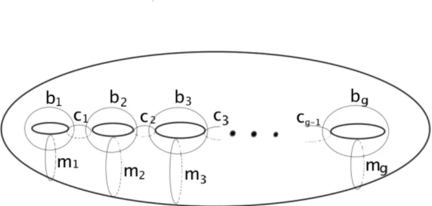
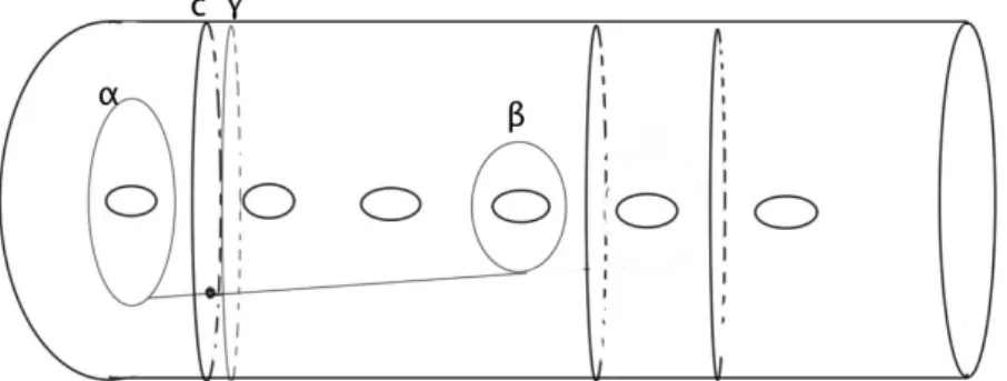
In particular, Proposition 2.1 tells you the size of a maximal collection of disjoint separating curves on S , as there is always a subgroup of rank rkK = rkI generated by Dehn

Keywords: continuous time random walk, Brownian motion, collision time, skew Young tableaux, tandem queue.. AMS 2000 Subject Classification: Primary:

Such simple formulas seem not to exist for the Lusztig q-analogues K λ,μ g (q) even in the cases when λ is a single column or a single row partition.. Moreover the duality (3) is

Answering a question of de la Harpe and Bridson in the Kourovka Notebook, we build the explicit embeddings of the additive group of rational numbers Q in a finitely generated group

Debreu’s Theorem ([1]) says that every n-component additive conjoint structure can be embedded into (( R ) n i=1 ,. In the introdution, the differences between the analytical and

We now show that the formation of the Harder-Narasimhan filtration commutes with base change, thus establishing the slope filtration theorem; the strategy is to show that a

We give a Dehn–Nielsen type theorem for the homology cobordism group of homol- ogy cylinders by considering its action on the acyclic closure, which was defined by Levine in [12]

In fact, the homology groups in the top 2 filtration dimensions for the cabled knot are isomorphic to the original knot’s Floer homology group in the top filtration dimension..