Realizing directional sound source in FDTD method by estimating initial value

(1)

Realizing directional sound source in FDTD method by estimating initial value

FDTD

法の初期値推定による指向性音源の実現

1W143070-1 竹内大起指導教員及川靖広教授

TAKEUCHI Daiki Prof. OIKAWA Yasuhiro

概要：波動音響シミュレーションにおいて指向性音源を扱うことは，実環境に近い予測・模擬をする上で重要な課題 である．波動方程式の時間領域解法では，音圧と粒子速度を初期値として与える手法が広く用いられている．この手法では，適当な初期値を与えれば，それに対応した音波伝搬を得られる．もし，音波伝搬に特定の指向性を与える初期値が存在するならば，それを求めることで

FDTD

法にその指向性を導入できる．そこで本研究では，

FDTD

法の行列表現を用いて，任意の指向性パターンから，その指向性を持つ音波伝搬を与える初期値を推定する手法を提案する．また，得られた初期値の時間発展を

FDTD

法で計算し，所望の指向性を導入できていることを確認した．

キーワード：指向性音源、波動音響シミュレーション、時間領域有限差分法、最小二乗法、クリロフ部分空間法

Keywords: sound source directivity, wave-based acoustic simulation, finite-diﬀerence time-domain (FDTD), least squares method, Krylov subspace method.

1. Introduction

Wave-based acoustic simulation methods are studied actively for predicting acoustical phenomena. Finite- diﬀerence timedomain (FDTD) method is one of the most popular methods owing to its straightforwardness of calcu- lating an impulse response. In an FDTD simulation, an omnidirectional sound source is usually adopted, which is not realistic because the real sound sources often have spe- cific directivities. However, there is very little research on imposing a directional sound source into FDTD methods.

In this thesis, a method of realizing a directional sound source in FDTD methods is proposed[1]. It is formulated as an estimation problem of the initial value so that the estimated result approximates the desired directivity. The eﬀectiveness of the proposed method is illustrated through some numerical experiments.

2. Finite-diﬀerence time-domain method

In 2-D acoustic field, diﬀerence formula of FDTD method can be written as

u

^[n+1]_i,j

= u

^[n]_i,j

− ∆t ρ∆h

{

p

^[n]_i,j

− p

^[n]_i₋_1,j

}

, (1)

v

_i,j^[n+1]

= v

^[n]_i,j

− ∆t ρ∆h

{

p

^[n]_i,j

− p

^[n]_i,j₋₁

}

, (2)

p

^[n+1]_i,j

= p

^[n]_i,j

− κ∆t

∆h [{

u

^[n+1]_i+1,j

− u

^[n+1]_i,j

} + {

v

_i,j+1^[n+1]

− v

_i,j^[n+1]

}]

, (3)

where p

^[n]_i,j

is sound pressure, u

^[n]_i,j

and v

_i,j^[n]

is particle ve- locities in x and y directions, respectively, ρ is density, κ is bulk modulus, ∆t is a discrete time step, ∆h is the size of the staggered grid, and n, i and j are indices of the time step, spatial steps of x and y, respectively[2]. This scheme takes advantage of the staggered grid which enables im- plementation of the central finite difference in the form of the forward or backward finite differences. The number of time sequences is chosen so that the initial wave does not reach to the boundary for avoiding the effect of boundary condition where properly choosing it is not easy.

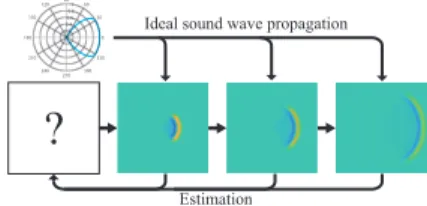
Since any recursive scheme starts its iteration from an initial value (p, u, v at n = 0), it decides the behavior of the initial wave propagation. That is, the directivity of a sound source is totally decided by the initial value. Thus, in this situation, the approximation of the desired directivity can be formulated as a problem of finding the corresponding initial value. However, setting an appropriate initial condition which generates the desired directivity pattern is a challenging task because it should depend on the choice

Fig. 1 Estimating initial value from a directional pattern.

The initial value is estimated from a propagated wave with the desired directivity pattern which is ideally cre- ated from the given pattern by multiplication.

of an FDTD scheme. Therefore, a method of imposing a directional sound source that is independent of choosing a scheme is necessary.

3. Proposed method

As discussed in the previous section, a directional sound source can be realized by obtaining the corresponding initial value of an FDTD method. To do so, an initial value estimation method is proposed. The main idea of the proposed method is illustrated in Fig. 1. Since it is formulated as a least squares problem, a matrix representation of the FDTD method is introduced first.

3. 1 Matrix representation of FDTD method For each time step n, vectors p

^[n]

∈ R

^N^p²

, u

^[n]

∈ R

^N^p^(N^p⁺¹⁾

and v

^[n]

∈ R

^(N^p^+1)N^p

are defined so that all (i, j)-th values of p, u and v are contained in the corresponding vectors. By these notations, the update rule of the FDTD method in Eqs. (1), (2) and (3) can be inter- preted as a linear transformation from (p

^[n]

,u

^[n]

, v

^[n]

) to (p

^[n+1]

, u

^[n+1]

, v

^[n+1]

), which can be explicitly written as

u

^[n+1]

= u

^[n]

+ ∆t

ρ D

_x^T

p

^[n]

, (4)

v

^[n+1]

= v

^[n]

+ ∆t

ρ D

_y^T

p

^[n]

, (5)

p

^[n+1]

= p

^[n]

− κ∆t (

D

x

u

^[n+1]

+ D

y

v

^[n+1]

) , (6) where D

x

, D

y

∈ R

^N^p²^×^N^p^(N^p⁺¹⁾

are the diﬀerence oper- ators in x and y directions, respectively, and ·

^T

denotes transpose.

Let a state vector ζ

^[n]

at time step n be defined as ζ

^[n]

= [ p

^[n]T

, u

^[n]T

, v

^[n]T

]

^T

∈ R

^3N^p²^+2N^p

, where [z

1

, z

2

] is horizontal concatenation of z

1

and z

2

. Then, Eqs. (4), (5) and (6) can be compactly represented as

ζ

^[n+1]

= Φζ

^[n]

= Φ

ⁿ⁺¹

ζ

^[0]

, (7)

(2)

(a) (b)

Fig. 2 (a) Region of considering initial value (blue) and observation points for evaluating a directivity pattern (red).

(b) Example of sound pressure at the observation points which constructs d in Eq. (12).

where Φ is a block matrix of the form

Φ =



 

I − D − κ∆t D

x

− κ∆t D

y

∆t

ρ

D

_x^T

I O

∆t

ρ

D

_y^T

O I



  , (8)

I ∈ R

^(N^p²^+N^p⁾^×^(N^p²^+N^p⁾

and O ∈ R

^(N^p²^+N^p⁾^×^(N^p²^+N^p⁾

denotes the identity matrix and the zero matrix, respectively, and

D = κ(∆t)

²

ρ (D

x

D

^T_x

+ D

y

D

^T_y

). (9) This matrix representation in Eq. (7) shows that a single time step of the FDTD scheme is equivalent to multiplication of the matrix Φ to the state vector ζ

^[n]

. Using this representation, a least squares problem of the FDTD method can be formulated.

3. 2 Estimating initial value from directivity pattern

For realizing a directional sound source, a method for estimating the initial value corresponding to the desired directivity pattern is proposed here.

In the proposed method, the initial value is assumed to be compactly supported on a small region illustrated as a blue circle in Fig. 2(a). This assumption reflects the size of a directional sound source. After the initial value is propagated by an FDTD scheme, sound pressure around that region is expected to have the desired directivity. Therefore, observation points, illustrated as a red circle in Fig. 2(a), is set around the region, and directivity is evaluated at these points. The aim of the proposed method is to estimate the initial value supported inside the blue region so that the directivity evaluated at the red observation points approximates the desired directivity pattern.

The inverse problem of estimating an initial value is formulated as a least squares problem of the FDTD method. A vector of an initial value is defined as ξ = [ p

_in^T

, u

inT

, v

inT

]

^T

∈ R

^Nⁱⁿ

, where the length of ξ is much smaller than that of ζ

^[0]

because ξ only consists of the small region in Fig. 2(a). In a similar manner, a vector of sound pressure at the observation points is denoted by p

^[n]_pick

∈ R

^N^pick

whose length is also much smaller than that of ζ

^[n]

, and the relation is expressed as

p

^[n]_pick

= LΦ

ⁿ

Eξ, (10) where E : R

^Nⁱⁿ

→ R

^3N^p²^+2N^p

is a matrix that each column of E contains only single 1 and other elements are 0 and L : R

^3N^p²^+2N^p

→ R

^N^pick

is a matrix that each row contains only single 1 and other elements are 0. By concatenating each p

^[n]_pick

vertically as p

_pick

= [ p

^[1]_pick^T

, p

^[2]_pick^T

, . . . , p

^[n]_pick^T

]

^T

, a linear equation considering all time steps is obtained:

p

_pick

= L

diag

F Eξ, (11) where L

diag

= blkdiag(L, L, · · · , L) is the block diagonal matrix, blkdiag generates a block diagonal matrix from its arguments, and F = [ Φ

^T

, (Φ

²

)

^T

, · · · ,(Φ

ⁿ

)

^T

]

^T

. Then, an estimation problem of the initial value can be formulated as the following least squares problem: Finding

ˆ ξ = arg min

ξ

L

_diag

F Eξ − d

²

2

, (12)

0 30 90 60 120 150 180

210

240 270 300

330 0 0.20.40.60.81

0 30 90 60 120 150 180

210

240 270 300

330 0 0.20.40.60.81

0 30 90 60 120 150 180

210

240 270 300

330 00.2 0.40.60.81

Fig. 3 Propagated waves generated by estimated initial value in FDTD(2,2) method. Their directivities were evaluated at 2 m away from the center.

Fig. 4 Estimated initial value corresponding to Fig. 3 (b).

where d consists of pulse signals at the observation points as illustrated in Fig. 2(b). The desired directivity pattern is ideally imposed to d by multiplying it to received signals obtained by an omnidirectional pulse emitted from the center of the region of the initial value. By solving this problem, the initial value approximating the desired directivity is obtained.

4. Numerical experiment

Numerical experiments ware conducted in order to con- firm the appropriateness of the proposed method. In numerical experiment, size of sound field is 10 m × 10 m, initial value region is disk of radius 1 m and observation point is circle of radius 1.1 m. For solving the least squares problem in Eq. (12), the LSMR solver [3], which is a MINRES (Krylov subspace type method) variant of the well-known LSQR , was utilized.

Fig. 3 shows the results of propagated initial values which ware estimated by the proposed method. Each row corre- sponds to one of four diﬀerent directivity patterns, and the polar plots were normalized by their maximal values. From the time sequences of sound pressure and the polar plots of directivities, it can be confirmed that directional sound sources were realized by the proposed method. Fig. 4 shows the estimated initial value corresponding to Fig. 3 (b). It can be seen that manually setting such an initial value is not an easy task even when the desired directivity was a simple pattern.

5. Conclusions

In this thesis, the method of realizing directional sound sources by estimating the initial value of an FDTD method was proposed. The proposed method can approximately impose any directivity pattern in an automatic manner even when the corresponding initial value is complicated. In fu- ture work, the eﬀect of the setting of the region of the initial value and observation points should be investigated to achieve better performance. Moreover, the property of the matrix L

_diag

F E should be analyzed so that the ability of approximating directivity patterns by the initial value is understood.

References

[ 1 ] D. Takeuchi, K. Yatabe，Y. Oikawa，“Realizing directional sound source in FDTD method by estimating initial value,”in

IEEE Int. Conf. Acoust., Speech, Signal Process.

(ICASSP), Apr. 2018.

[ 2 ] D. Botteldooren, “Finite–diﬀerence time–domain simulation of low-‐frequency room acoustic problems,”

J. Acoust.

Soc. Am., vol. 98, no. 6, pp. 3302–3308, 1995.

[ 3 ] D. C. Fong and M. Saunders, “LSMR: An iterative al- gorithm for sparse least-squares problems,”

SIAM J. Sci.

Comput., vol. 33, no. 5, pp. 2950–2971, 2011.

Realizing directional sound source in FDTD method by estimating initial value