ModiﬁedBalancedAssignmentProbleminVectorCase 「幻想の帝国」

(1)

Modified Balanced Assignment Problem in Vector Case

– An Attempt to Apply the Method for 2-dimensional Case to 3-dimensional – Yuusaku Kamura

Abstract We consider a combinatorial problem that arises from systems’ construction. Each system consists of many components, and every component has its own error expressed in a vector. It is required to make the combination that minimizes as small as possible the difference between the maximum error and the minimum one. It means the vector case’s balanced optimization problem. In this paper, we deal with the case that each system consists of 2 components and the vector dimension is 3. We apply the approximation algorithm that we have presented for 2-dimensional case to 3-dimensional problem and we show the numerical experiments.

Keywords optimization; approximation algorithm; assignment problem; combinatorial problem 1. INTRODUCTION

Suppose we havensuppliersu1, u2, . . . , un (to be denoted by a setU) andncustomersv1, v2, . . . , vn

(to be denoted byV). If supplieruiand customervjare chosen, the cost iscij. We are going to determine a one to one correspondenceπ:U →V under an appropriate objective function. This is the well-known assignment problem.

Since making the one to one correspondence π : U → V is equivalent to permuting the set {1,2, . . . , n}, we hereafter call the one to one correspondence as permutation.

The assignment problem has various versions with respect to the objectives [1]. If we are going to minimize the total sum of the cost∑n

i=1ciπ(i), the problem is called thelinear sum assignment problem, and there have been proposed many efficient algorithms [2].

If we are going to minimize the difference of the maximum cost and the minimum one of the corresponded pair, the problem is called thebalanced assignment problem[3]. The objective is

minπ {max

1≤i≤nciπ(i)− min

1≤i≤nciπ(i)}. (1)

The polynomial time algorithms have been proposed for this problem, too.

In this paper we extend the balanced assignment problem to the case that costs are multidimensional, i.e., vectors. Here we assume that cost vectorcij is represented as a sum of the supplier vectorai and the customer vectorbj.

A formal description of our problem is as follows. Let A and B be sets of m dimensional vectors. We denote each element of A by ai = (a⁽¹⁾_i , a⁽²⁾_i , . . . , a^(m)_i ) and each element of B by bi = (b⁽¹⁾_i , b⁽²⁾_i , . . . , b^(m)_i ). We assume that a⁽¹⁾_i , a⁽²⁾_i , . . . , a^(m)_i and b⁽¹⁾_i , b⁽²⁾_i , . . . , b^(m)_i are nonnegative and define the sum of vectorsai+bj as

ai+bj = (a⁽¹⁾_i +b⁽¹⁾_j , a⁽²⁾_i +b⁽²⁾_j , . . . , a^(m)_i +b^(m)_j ). (2) We denote this vectors’ sum ascij, namelycij =ai+bj. Let us consider the following problem: find a permutationπof a set {1,2, . . . , n}such that

Tm(π) = max{ max_1≤i≤nc⁽¹⁾_iπ(i)−min_1≤i≤nc⁽¹⁾_iπ(i), max1≤i≤nc⁽²⁾_iπ(i)−min1≤i≤nc⁽²⁾_iπ(i),

...

max_1≤i≤nc^(m)_iπ(i)−min_1≤i≤nc^(m)_iπ(i)}

(3)

「幻想の帝国」

――日本と朝鮮半島のパラダイム――

重村智計

Abstract This article titled “Illusory Empire—Paradigm Between Japan and Korean Peninsula” focuses on how the academia in Japan and in two Koreas differ. The different perspectives derive from each nation’s prescribed perception which

accumulated over the years. Japan has its own image and interpretation built on its own academia. The Korean academia also constructed its interpretation on Japan as a subject from Korea’s own perception. Japan and Korea each has developed the logic of interpretation from its own illusion far from the objective analysis. For example, Japan’s interpretation of Korea-related issues would likely to be based on sources and references from the Japanese academia far from the Korea’s native stance.

A question like, “What is the origin of Korean war?” involves multiple disputes and arguments. One predominant analysis on the Korean War relies on North Korea’s accusation of the United States. The reasoning is that the U.S. invaded North Korea.

One research after another uses the circular reasoning based on the similar analysis.

Such analysis cannot be deemed as a true interpretation. North Korea invaded South Korea on may1950. After the collapse of the Cold War, official documents of Soviet Russia disclosed facts that North Korea crossed over the 38 parallel which was a geographical division between South and North Korea. There are false interpretations regarding Korean issues. This article analyses such false facts and argue against self-referenced theories. This article aims to clarify the truth implementing theories of international relations.

The Korea Study have been referred to “regional studies”, which includes themes related to history, culture, religion, philosophy. This article uses mainly the

constructive theory from the international theories.

Korea: the Politics of the Vortex written by Gregory Henderson, a former Professor at Harvard University, is one of the classics in Korean Studies. Henderson addresses the notion of vortex society and politics in the Korean peninsula. Henderson

characterizes the Korean political system and culture as a centralized governance for nearly 2000 years. This article analyzes illusory interpretation and facts of South and North Korea. The ultimate objective of this article is to seek and confirm the truth.

(2)

is the minimum.Tm(π)means the maximum of mdifferences

1max≤i≤nc^(k)_iπ(i)− min

1≤i≤nc^(k)_iπ(i), (4)

where1≤k≤m.

Such a problem appears when we combine industrial products. Each system consists of many individ- uals. The lens for a semiconductor manufacturing system is such a product. That includes many lenses (about30) and the error of each one is given by the high dimensional vector.

Fig. 1. System construction. A system consists oflcomponentsCi(i= 1,2, . . . , l). Each component is given by the lot.

It is required to minimize the variation range of systems’ errors. That problem is generally formulated to a multi-index balanced assignment problem. But it is shown that even a multi-index linear sum assignment in scalar case is NP-complete. Therefore for the vector case’s balanced assignment problem, we deal with the problem in a single-index, that is, the combination between2 sets ofnvectors.

From the above assumptions, our problem is formulated as follows:

Problem 1 Given2 sets ofn vectorsAandB, find the permuationπ that minimizes Tm(π) = max

1≤k≤m{max

i c^(k)_iπ(i)−min

i c^(k)_iπ(i)}, (5)

wherec^(k)_iπ(i)=a^(k)_i +b^(k)_π(i).

In our former research [4], [5], [6], [7] we considered the problem of makingnsets of system such that the worst combined error is the minimum. On the other hand, in [8] we dealt with the balanced assignment problem in 2-dimensional vector case. In this paper we attempt to apply our algorithm in [8]

to the problem in 3-dimensional vector case.

Remark In general assignment problems, edges’ costs are given independently. However, in our problem they are introduced by the vertices’ costs. Hence we call this the ‘modified’ problem.

2. FORMULATION AS AN INTEGER PROGRAMMING PROBLEM

Problem 1 is formulated to the following 0-1 integer programming problem. HereM is a sufficient big number.

Problem 2 Minimizef =t subject to

u^(k)−l^(k)≤t, (k= 1,2, . . . , m);

(3)

c^(k)_ij xij ≤u^(k), (i, j= 1,2, . . . , n;k= 1,2, . . . , m);

l^(k)≤c^(k)_ij xij+M(1−xij), (i, j= 1,2, . . . , n;k= 1,2, . . . , m);

∑n

i=1

xij = 1, (j= 1,2, . . . , n);

∑n

j=1

xij = 1, (i= 1,2, . . . , n);

l^(k)≥0, u^(k)≥0, (k= 1,2, . . . , m);

xij ∈ {0,1}, (i, j= 1,2, . . . , n).

Unlike the scalar case’s assignment problem, no polynomial time algorithm exists to obtain the integer solution of this problem, and unfortunately, the relaxation method is not effective for this type of integer programming problems [9]. So instead of trying to solve Problem 2 directly, we propose an approximation algorithm which gives a quasi optimal solution.

3. PROPERTY OF THE PROBLEM

Before describing our algorithm for Problem 1, let us consider the property of our problem.

At first, let us consider the case thatm= 1, i.e.,ai andbj are scalars. It is trivial that the total sum ofciπ(i) does not depend onπ, i.e.,

∑n

i=1

ciπ(i)=

∑n

i=1

ai+

∑n

i=1

bπ(i)=

∑n

i=1

ai+

∑n

j=1

bj =const. (6)

Next, let us consider the case that m = 3. In this case again the total sum of c⁽¹⁾_iπ(i) and that of c⁽²⁾_iπ(i),c⁽³⁾_iπ(i)do not depend onπ. We denote ¹_n∑n

i=1(a⁽¹⁾_i +b⁽¹⁾_i )byµ1and ¹_n∑n

i=1(a⁽²⁾_i +b⁽²⁾_i )byµ2,

1 n

∑n

i=1(a⁽³⁾_i +b⁽³⁾_i )by µ3. For generalm, the situation is unchanged.

Thus, we have the following Property 1.

Property 1 For eachk, the total sum ofc^(k)_iπ(i)does not depend on the selection of permutationπand is constant.

4. ALGORITHM FORPROBLEM1

Hereafter we consider the case that the dimension of error vector is3. So we rewrite our proposed algorithm for 2-dimensional case in [8] to 3-dimensional case.

Firstly, we assume the following two properties.

Assumption 1

(i) Each vector’s dimension is3, that is, m= 3.

(ii)µ1=µ2=µ3. We denote itµ.

Our proposed algorithm uses the searching method of scalar case’s in [3]. It is the procedure that narrows gradually the range of edges’ weight which restricts edges to be used to construct a complete matching betweenA andB.

We describe the essence of the searching method.

Searching method

C= (cij)i,j=1,2,...,n : the cost matrix for ann×nassignment problem.

v1< v2<· · ·< vk : the values appearing inC.

l : the smallest value’s number ofvi.u: the largest one.

eij : the edge corresponds to cij. whileu < k do

begin is the minimum.Tm(π)means the maximum of mdifferences

1max≤i≤nc^(k)_iπ(i)− min

1≤i≤nc^(k)_iπ(i), (4)

where1≤k≤m.

Such a problem appears when we combine industrial products. Each system consists of many individ- uals. The lens for a semiconductor manufacturing system is such a product. That includes many lenses (about30) and the error of each one is given by the high dimensional vector.

Fig. 1. System construction. A system consists oflcomponentsCi(i= 1,2, . . . , l). Each component is given by the lot.

It is required to minimize the variation range of systems’ errors. That problem is generally formulated to a multi-index balanced assignment problem. But it is shown that even a multi-index linear sum assignment in scalar case is NP-complete. Therefore for the vector case’s balanced assignment problem, we deal with the problem in a single-index, that is, the combination between2 sets ofnvectors.

From the above assumptions, our problem is formulated as follows:

Problem 1 Given 2sets of nvectorsAandB, find the permuation πthat minimizes Tm(π) = max

1≤k≤m{max

i c^(k)_iπ(i)−min

i c^(k)_iπ(i)}, (5)

wherec^(k)_iπ(i)=a^(k)_i +b^(k)_π(i).

In our former research [4], [5], [6], [7] we considered the problem of makingnsets of system such that the worst combined error is the minimum. On the other hand, in [8] we dealt with the balanced assignment problem in 2-dimensional vector case. In this paper we attempt to apply our algorithm in [8]

to the problem in 3-dimensional vector case.

Remark In general assignment problems, edges’ costs are given independently. However, in our problem they are introduced by the vertices’ costs. Hence we call this the ‘modified’ problem.

2. FORMULATION AS AN INTEGER PROGRAMMING PROBLEM

Problem 1 is formulated to the following 0-1 integer programming problem. HereM is a sufficient big number.

Problem 2 Minimize f =t subject to

u^(k)−l^(k)≤t, (k= 1,2, . . . , m);

(4)

if eijs satisfy vl≤w(eij)(=cij)≤vu can create a complete matching then

l←l+ 1 else

u←u+ 1;

end;

For the scalar case, the complexity of checking whether a complete matching exists isO(n^2.5)[10], and the above search step is iteratedn²times in the worst case, hence it is easy to see that the total time complexity of the algorithm isO(n^4.5). Furthermore, there has been proposed an O(n⁴)algorithm [3].

A. Basis and idea for the 3-dimensional case

From Property 1, the best π is combining each c^(k)_iπ(i)(= a^(k)_i +b^(k)_π(i)) as closer to the mean µ as possible.

We normalize eacha⁽¹⁾_i and represent it as˜a⁽¹⁾_i , that is,

˜

a⁽¹⁾_i =a⁽¹⁾_i −µa1

σa1

, (7)

where σa1 is the variance of a⁽¹⁾_i s and µa1 is the mean of them. By the normalization a⁽¹⁾_i is converted to the probabilistic variable that the mean and the variance is 0 and 1, respectively. We define

˜

a⁽²⁾_i ,˜a⁽³⁾_i ,˜b⁽¹⁾_j ,˜b⁽²⁾_j ,˜b⁽³⁾_j similarly.

So we can say that c^(k)_iπ(i) = a^(k)_i +b^(k)_π(i) = µ is equivalent to ˜a^(k)_i + ˜b^(k)_π(i) = 0. Our problem is converted to find the permutationπ: {1,2, . . . , n} → {1,2, . . . , n} that all 3n values ˜a⁽¹⁾_i + ˜b⁽¹⁾_π(i) and

˜

a⁽²⁾_i + ˜b⁽²⁾_π(i),a˜⁽³⁾_i + ˜b⁽³⁾_π(i) are as close to origin as possible (Fig.2. Illustrate2-dimensional case).

Fig. 2. 2-dimensional case : find a permutationπthat combines each(˜a⁽¹⁾_i ,˜a⁽²⁾_i )to(˜b⁽¹⁾_π(i),˜b⁽²⁾_π(i))such that those of center to be as close to origin as possible. Similar for the 3-dimensional case.

From this fact, we consider the assignment problem whose objective is g=

∑n

i=1

max{

|ã⁽¹⁾_i + ˜b⁽¹⁾_π(i)|,|ã⁽²⁾_i + ˜b⁽²⁾_π(i)|,|ã⁽³⁾_i + ˜b⁽³⁾_π(i)|}

. (8)

To minimize g, it is sufficient to minimize

|˜a⁽¹⁾_i + ˜b⁽¹⁾_π(i)| and |˜a⁽²⁾_i + ˜b⁽²⁾_π(i)|, |a˜⁽³⁾_i + ˜b⁽³⁾_π(i)|. (9) Therefore we can expectπthat minimizesggives an approximate solution to Problem 1. The assignment problem forg is a linear sum assignment problem, which is easy to solve.

(5)

And we construct a cost matrix C˜ for searching, where the element of C˜ is the maximum value of

˜

cij = max{|˜a⁽¹⁾_i + ˜b⁽¹⁾_j |,|a˜⁽²⁾_i + ˜b⁽²⁾_j |,|˜a⁽³⁾_i + ˜b⁽³⁾_j |}. (10) B. Algorithm

Outline of our proposed algorithm is as follows:

(i) According to the searching method of scalar case’s algorithm, forvl≤˜cij ≤vu, in order to get the permutationπ, solve the linear sum assignment problem for g.

(ii) For Problem 1 ifπgives better solution than the previous one, adoptπas the provisional best solution π^∗.

(iii) Narrow the range[vl, vu], then go to (i).

Now in the following Algorithm 1 we show in detail our proposed algorithm.

Algorithm 1

Preparation(Create a cost matrix) Define the cost matrixC˜= (˜cij)by

˜

cij = max{|˜a⁽¹⁾_i + ˜b⁽¹⁾_j |,|a˜⁽²⁾_i + ˜b⁽²⁾_j |,|˜a⁽³⁾_i + ˜b⁽³⁾_j |}. (11) v1< v2<· · ·< vk : the values appear inC.˜

C(l, u)˜ : the set of˜cij satisfies vl≤˜cij ≤vu. T3(π): defined in (3) wherem= 3.

Step0 (Initialization) l←1, u←1, t← ∞.

Step1 (Set edges’ weightswij and solve the linear assignment problem) for i←1 to n do

begin

for j←1 to n do begin

if vl≤˜cij ≤vu then

wij ←max{˜a⁽¹⁾_i + ˜b⁽¹⁾_j ,a˜⁽²⁾_i + ˜b⁽²⁾_j ,˜a⁽³⁾_i + ˜b⁽³⁾_j } else wij ← ∞;

end;end;

Solve the linear assignment problem forwij : g=∑n

i=1

∑n

j=1wijxij,then

if g̸=∞ then goto Step 2 else goto Step 3;

Step2 (C(l, u)˜ contains a complete matching) if l=u then

begin

T ←0;l^∗←u^∗;u^∗←u; stop elseend

begin

if T > T3(π) then begin

T ←T3(π);π^∗←π;l^∗←l;u^∗←u end;

ifeijs satisfy vl≤w(eij)(=cij)≤vu can create a complete matching then

l←l+ 1 else

u←u+ 1;

end;

For the scalar case, the complexity of checking whether a complete matching exists isO(n^2.5)[10], and the above search step is iteratedn²times in the worst case, hence it is easy to see that the total time complexity of the algorithm isO(n^4.5). Furthermore, there has been proposed an O(n⁴)algorithm [3].

A. Basis and idea for the 3-dimensional case

From Property 1, the best π is combining each c^(k)_iπ(i)(= a^(k)_i +b^(k)_π(i)) as closer to the mean µ as possible.

We normalize each a⁽¹⁾_i and represent it as˜a⁽¹⁾_i , that is,

˜

a⁽¹⁾_i =a⁽¹⁾_i −µa1

σa1

, (7)

where σa1 is the variance of a⁽¹⁾_i s and µa1 is the mean of them. By the normalization a⁽¹⁾_i is converted to the probabilistic variable that the mean and the variance is 0 and1, respectively. We define

˜

a⁽²⁾_i ,˜a⁽³⁾_i ,˜b⁽¹⁾_j ,˜b⁽²⁾_j ,˜b⁽³⁾_j similarly.

So we can say that c^(k)_iπ(i) = a^(k)_i +b^(k)_π(i) = µ is equivalent to ˜a^(k)_i + ˜b^(k)_π(i) = 0. Our problem is converted to find the permutationπ: {1,2, . . . , n} → {1,2, . . . , n} that all 3nvalues ˜a⁽¹⁾_i + ˜b⁽¹⁾_π(i) and

˜

a⁽²⁾_i + ˜b⁽²⁾_π(i),˜a⁽³⁾_i + ˜b⁽³⁾_π(i) are as close to origin as possible (Fig.2. Illustrate2-dimensional case).

Fig. 2. 2-dimensional case : find a permutationπthat combines each(˜a⁽¹⁾_i ,˜a⁽²⁾_i )to(˜b⁽¹⁾_π(i),˜b⁽²⁾_π(i))such that those of center to be as close to origin as possible. Similar for the 3-dimensional case.

From this fact, we consider the assignment problem whose objective is g=

∑n

i=1

max{

|ã⁽¹⁾_i + ˜b⁽¹⁾_π(i)|,|ã⁽²⁾_i + ˜b⁽²⁾_π(i)|,|ã⁽³⁾_i + ˜b⁽³⁾_π(i)|}

. (8)

To minimizeg, it is sufficient to minimize

|˜a⁽¹⁾_i + ˜b⁽¹⁾_π(i)| and |˜a⁽²⁾_i + ˜b⁽²⁾_π(i)|, |a˜⁽³⁾_i + ˜b⁽³⁾_π(i)|. (9) Therefore we can expectπthat minimizesggives an approximate solution to Problem 1. The assignment problem forg is a linear sum assignment problem, which is easy to solve.

(6)

l←l+ 1; goto Step 1 end;

Step3 (C(l, u)˜ does not contain a complete matching) if u=k then stop

elsebegin

u←u+ 1; goto Step 1 end;

When Algorithm 1 terminated,π^∗ gives the quasi optimal solution to Problem 1.

The time complexity of Algorithm 1 isO(n⁵). Because Algorithm 1 solves the linear sum assignment problemn²times. The linear sum assignment problem can be solved inO(n³) [2].

5. NUMERICAL EXPERIMENTS

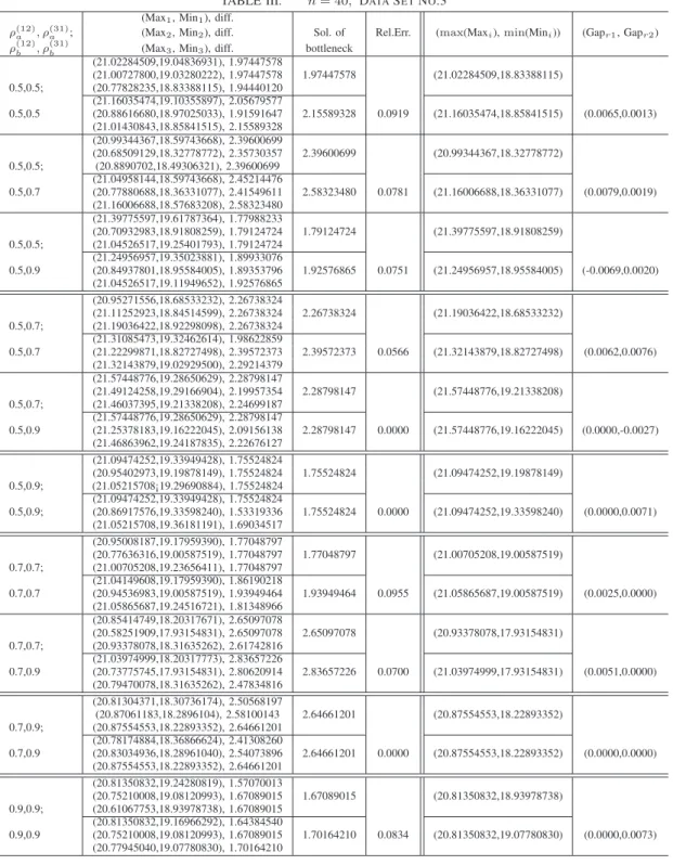
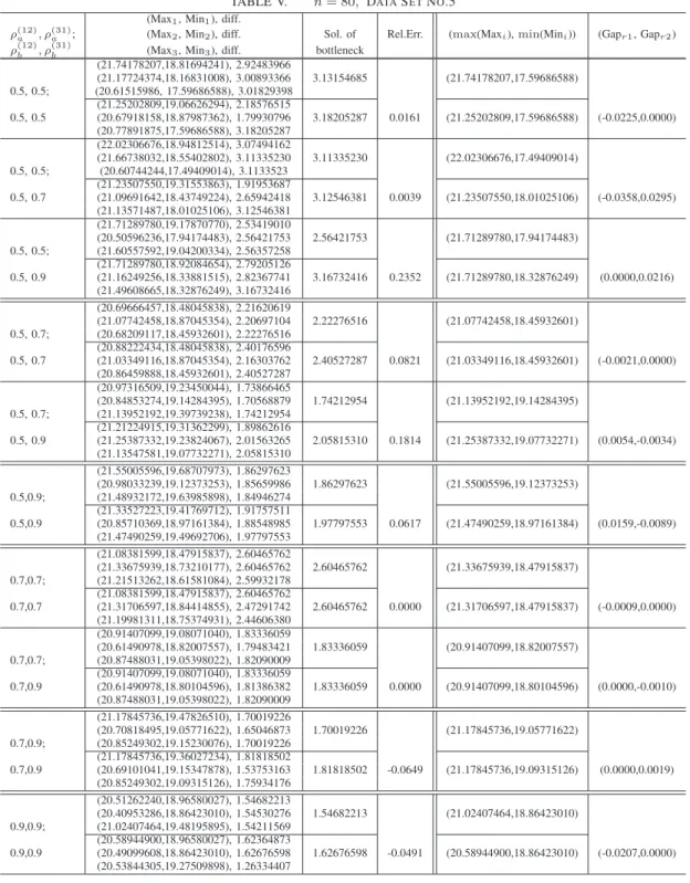
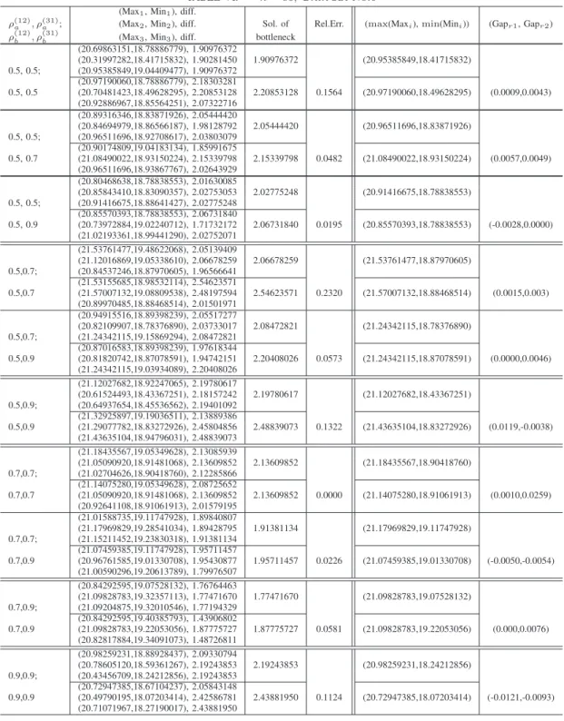
We prepare the test data for the numerical experiments as follows : For vectorsai= (a⁽¹⁾_i , a⁽²⁾_i , a⁽³⁾_i ) and bj = (b⁽¹⁾_j , b⁽²⁾_j , b⁽³⁾_j ), (i, j = 1,2, . . . , n), let a⁽¹⁾_i , a⁽²⁾_i , a⁽³⁾_i ; b⁽¹⁾_j , b⁽²⁾_j , b⁽³⁾_j follow the normal distribution that the mean is10and the variance is1, respectively. Hereρ⁽¹²⁾a is the correlation coefficient of a⁽¹⁾_i anda⁽²⁾_i ,ρ⁽³¹⁾a is that of a⁽³⁾_i anda⁽¹⁾_i . Similarly we define ρ⁽¹²⁾_b and ρ⁽³¹⁾_b . When the number of vectorsn is not so large, that is, at most 1000,0 ≤ρ⁽¹²⁾a <0.5 means the a⁽¹⁾_i anda⁽²⁾_i have little correlative relation. So ifn≤100, we can say that it is sufficient to setρ⁽¹²⁾a to0.5,0.7, and 0.9. It is the same forρ⁽³¹⁾a andρ⁽¹²⁾_b ,ρ⁽³¹⁾_b .

Each pair ofρ⁽¹²⁾a andρ⁽³¹⁾a ,ρ⁽¹²⁾_b andρ⁽³¹⁾_b , we prepare several different data sets forn= 40,80,120.

For each data set, we solve the problem by Algorithm 1, then compare to the exact solution. Exact solutions are found by solving Problem 1, that is the mixed integer programming problem(MIP), using the solver SCIP¹. We denote three results here forn= 40,80,120, respectively. Table I-III show in the casen= 40and also Table IV-VI show in the casen= 80, Table VII-IX show in the case n= 120.

In every two rows, the upper is the exact solution and the lower is the approximate one. The column

‘Sol. of bottleneck’ shows the solution to the problem. ‘Rel. Err.’ expresses the relative error of the approximate solution and the exact one, that is,

(Approximate solution by Algorithm 1)−(Exact solution)

(Exact solution) .

For the problem that minimizes each sum of elements, from ‘Rel. Err.’ we find our proposed algorithm does not give well approximate solutions to all cases. We think the result depends on the data’s property.It is not only the correlation coefficient.

But if we take max(Maxi);i = 1,2,3 and min(Minj);j = 1,2,3 , and we consider the interval [min(Minj),max(Maxi)]for exact solutions and approximate ones respectively, the two intervals almost coincide in every case. This is another bottleneck assignment problem formulated as Problem 3, that is, find the minimum interval includes 3 ones.

Problem 3 Given2 sets ofn vectorsAandB, find the permutation πthat minimizes T˜m(π) = max{ max

1≤k≤mmax

i c^(k)_iπ(i)− min

1≤k≤mmin

i c^(k)_iπ(i)}, (12)

wherec^(k)_iπ(i)=a^(k)_i +b^(k)_π(i). Here m= 3.

We also show the results of Problem 3 in each table. We define relative errors for the maximum value and the minimum one as follows:

Gap_r1 = Approx.max(Maxi)−Exact.max(Maxi) Exact.max(Maxi) , Gap_r2 = Approx.min(Mini)−Exact.min(Mini)

Exact.min(Mini) .

1SCIP (Solving Constraint Integer Programs) is a non-commercial MIP solver developed at Zuse Institute Berlin. http://scip.zib.de/

(7)

We find Gap_r1,Gap_r2 are less than5% in almost every case. So we can say that our algorithm is efficient for Problem 3.

A. Considerations

From numerical experiments, unfortunately our proposed algorithm is not always efficient for the original 3-dimensional bottleneck assignment problem. Why the approximate solutions by our algorithm in each interval’s case is not good?

We think the reason is that when we create the cost matrix for searching, we take the representative inmax{c⁽¹⁾_ij , c⁽²⁾_ij , c⁽³⁾_ij }. Therefore the results are probably influenced by the maximum element.

For the original problem whose objective is to minimize each sum, how should we extend our method?

One idea is that we do not create only one searching matrix but 3 ones, and narrow the 3 ranges independently. But when we manipulate 3 searching matrices, the other difficulties will occur.

l←l+ 1; goto Step 1 end;

Step3 (C(l, u)˜ does not contain a complete matching) if u=k then stop

elsebegin

u←u+ 1; goto Step 1 end;

When Algorithm 1 terminated,π^∗ gives the quasi optimal solution to Problem 1.

The time complexity of Algorithm 1 isO(n⁵). Because Algorithm 1 solves the linear sum assignment problemn² times. The linear sum assignment problem can be solved inO(n³) [2].

5. NUMERICAL EXPERIMENTS

We prepare the test data for the numerical experiments as follows : For vectorsai= (a⁽¹⁾_i , a⁽²⁾_i , a⁽³⁾_i ) and bj = (b⁽¹⁾_j , b⁽²⁾_j , b⁽³⁾_j ), (i, j = 1,2, . . . , n), let a⁽¹⁾_i , a⁽²⁾_i , a⁽³⁾_i ; b⁽¹⁾_j , b⁽²⁾_j , b⁽³⁾_j follow the normal distribution that the mean is10and the variance is1, respectively. Hereρ⁽¹²⁾a is the correlation coefficient of a⁽¹⁾_i anda⁽²⁾_i ,ρ⁽³¹⁾a is that of a⁽³⁾_i anda⁽¹⁾_i . Similarly we define ρ⁽¹²⁾_b andρ⁽³¹⁾_b . When the number of vectorsn is not so large, that is, at most 1000,0 ≤ρ⁽¹²⁾a <0.5 means the a⁽¹⁾_i anda⁽²⁾_i have little correlative relation. So ifn≤100, we can say that it is sufficient to setρ⁽¹²⁾a to0.5,0.7, and 0.9. It is the same forρ⁽³¹⁾a andρ⁽¹²⁾_b ,ρ⁽³¹⁾_b .

Each pair ofρ⁽¹²⁾a andρ⁽³¹⁾a ,ρ⁽¹²⁾_b andρ⁽³¹⁾_b , we prepare several different data sets forn= 40,80,120.

For each data set, we solve the problem by Algorithm 1, then compare to the exact solution. Exact solutions are found by solving Problem 1, that is the mixed integer programming problem(MIP), using the solver SCIP¹. We denote three results here forn= 40,80,120, respectively. Table I-III show in the casen= 40and also Table IV-VI show in the casen= 80, Table VII-IX show in the casen= 120.

In every two rows, the upper is the exact solution and the lower is the approximate one. The column

‘Sol. of bottleneck’ shows the solution to the problem. ‘Rel. Err.’ expresses the relative error of the approximate solution and the exact one, that is,

(Approximate solution by Algorithm 1)−(Exact solution)

(Exact solution) .

For the problem that minimizes each sum of elements, from ‘Rel. Err.’ we find our proposed algorithm does not give well approximate solutions to all cases. We think the result depends on the data’s property.It is not only the correlation coefficient.

But if we take max(Maxi);i = 1,2,3 and min(Minj);j = 1,2,3 , and we consider the interval [min(Minj),max(Maxi)]for exact solutions and approximate ones respectively, the two intervals almost coincide in every case. This is another bottleneck assignment problem formulated as Problem 3, that is, find the minimum interval includes 3 ones.

Problem 3 Given 2sets of nvectorsAandB, find the permutation πthat minimizes T˜m(π) = max{ max

1≤k≤mmax

i c^(k)_iπ(i)− min

1≤k≤mmin

i c^(k)_iπ(i)}, (12)

wherec^(k)_iπ(i)=a^(k)_i +b^(k)_π(i). Herem= 3.

We also show the results of Problem 3 in each table. We define relative errors for the maximum value and the minimum one as follows:

Gap_r1 = Approx.max(Maxi)−Exact.max(Maxi) Exact.max(Maxi) , Gap_r2 = Approx.min(Mini)−Exact.min(Mini)

Exact.min(Mini) .

1SCIP (Solving Constraint Integer Programs) is a non-commercial MIP solver developed at Zuse Institute Berlin. http://scip.zib.de/