- 152 - IEEE Workshop on Nonlinear Circuit NetworksDecember 9-10, 2011

Assessment of Stability for Oscillatory Circuit by Using Spice

Hiroshige Kataoka, Yoko Uwate, Yoshihiro Yamagami and Yoshifumi Nishio Department of Electrical and Electronic Engineering

Tokushima University Tokushima, Japan

Email: { hiroshige, uwate, yamagami, nishio } @ee.tokushima-u.ac.jp

Abstract— SPICE is a very convenient tool for circuit simula- tion and is used by many researchers. Nowadays, various SPICE- oriented algorithm are proposed. By using these methods, we can extend a function of SPICE and can analyze various circuit.

In this study, we propose a SPICE-oriented algorithm for assessment of stability for oscillatory circuit. We combine the har- monic balance method, Newton homotopy method and Floquet theory. We find out a oscillatory parameter by using harmonic balance method and Newton homotopy method, and we assess the stability by applying our method. As an example, we assess the stability of the periodic solutions for Cauer oscillator. The result shows our propose method gives the correct results.

I. I NTRODUCTION

SPICE is used for various analysis of the electrical circuit.

For example, AC analysis, DC analysis, sensitivity analysis, transient analysis etc. In addition, we can easily perform a SPICE simulation. We only have to make a netlist or schematic by computer, without writing a complex program. From this reason, many people use SPICE for circuit simulation. On the other hand, many researchers have proposed SPICE simulation method, which is the introduction of analytical dynamics. We propose a SPICE-oriented algorithm by applying the analytical dynamics and combine to the conventional method.

For designing oscillatory circuit, it is important to the assessment of the stability. We have proposed a SPICE- oriented algorithm to the assessment of the stability for pe- riodic solutions which is based on the Floquet theory [1]. In the conventional method, we assessed the stability of resonant circuit. In this study, we apply the our method to the oscillatory circuit by combining the Newton homotopy method [2]-[4].

The article is organized as follows. Section II-A shows how to use the sine-cosine circuits [5], which is based on the HB (harmonic balance) [6]-[8] method. We use the sine- cosine circuit to obtain the value of the voltages which are required in order to solve variational circuits. Section II-B shows the Newton homotopy method. This method is realized by using solution-curve tracing circuit(STC) [9]. Section II- C shows the Floquet theory [8][10]. Section III shows an illustrative example and how to solve the variational circuits by using SPICE. Section IV shows the results and confirms the effectiveness of the proposed method. Section V concludes this article.

II. SPICE-O RIENTED ANALYSIS OF OSCILLATOR

A. Sine-Cosine Circuit

The sine-cosine circuit has been introduced in order to solve the determining equations of the harmonic balance method by using SPICE. In this section, we explain how we can derive the sine-cosine circuit for simple passive element cases.

First, we set a voltage and a current with Fourier series;

 

 

 

 

 



v = V 0 +

∑ n k=1

(V s

_k

sin kωt + V c

_k

cos kωt)

i = I ₀ +

∑ n k=1

(I _s

_k

sin kωt + I _c

_k

cos kωt)

(1)

A current through a capacitor is given by i = C dv

dt . (2)

From Eqs. (1) and (2), we can express the current as i =

∑ n k=1

( − kωCV c

_k

sin kωt + kωCV s

_k

cos kωt). (3) From Eq. (3), we can express the relation between the coeffi- cients of sine and cosine components as follows;

{ I s

_k

= − kωCV c

_k

I c

_k

= kωCV s

_k

(4) In the case of an inductor, we can express the voltage across an inductor as

v =

∑ n k=1

( − kωLI c

_k

sin kωt + kωLI s

_k

cos kωt), (5) where the current through an inductor is given by

v = L di

dt . (6)

Equations for coefficient of sin kωt and cos kωt are given by { V _s

_k

= − kωLI _c

_k

V _c

_k

= kωLI _s

_k

. (7)

If we make the circuit model satisfying this method, a capacitor is replaced by coupled voltage-controlled current sources and an inductor is replaced by coupled current- controlled voltage sources in the sine-cosine circuit.

- 152 -

IEEE Workshop on Nonlinear Circuit Networks

December 9-10, 2011

B. Newton Homotopy Method

Newton homotopy method is one of method for finding multiple dc solutions. The circuit model of Newton homotopy method is shown in Fig. 1. We assume equations as follows;

 

 

 

 

 

 

 



g ₀ (V ₀ , V ₁ , V ₂ , . . . , V _M ) = 0 g 1 (V 0 , V 1 , V 2 , . . . , V M ) = 0 g 2 (V 0 , V 1 , V 2 , . . . , V M ) = 0 . . . .

g M − 1 (V 0 , V 1 , V 2 , . . . , V M ) = 0 g M (V 0 , V 1 , V 2 , . . . , V M ) = 0

. (8)

These determining equations are described by a set of al- gebraic equations, which consists of M -equations and same number of variables. However, it is not easy to solve the equations, because they may have the multiple solutions.

Applying the Newton homotopy method to solve Eq. (8), we obtain the following relation;

G(V , ρ) = g(V ) − (1 − ρ)g(V ₍₀₎ ) = 0. (9) where the initial state is set by a point (V ₍₀₎ , ρ = 0) and gets the solutions satisfying g(v) = 0 at ρ = 1 on the path. ρ shows solutions curves called homotopy paths, and find the multiple solutions lying on the paths. A solution curve is traced by ark-length method as follows;

 

 

 



 

 

 

G(V , ρ) = 0

∑ ( M dV i

ds ) 2

+ ( dρ

ds ) 2

= 1

i = 1 i ̸ = 2

. (10)

Equation (10) is realized by using ABMs. Figure 2 shows the circuit diagram of solution-curve tracing circuit (STC).

VCCS

VCCS

) 0 ( g 0

(0) g

¹

VCCS

) 0 ( g M )

0

(V, ρ g

)

1

(V, ρ g

ρ ) (V, g

^M

] 1[ Ω

STC ρ (0)

g 1) -

( ρ

⁰

(0) g 1) - ( ρ

¹

(0) g 1) -

( ρ

M

Σ

v

0

v

1

v

M

1 -

・

・

・

・

・

・

] 1[ Ω

] 1[ Ω

Fig. 1. Circuit model of Newton homotopy method.

2 1

∑

i M

M

i=

v

=

I &

ρ

v &

v ρ R

int 1[A]

ρ2

v

=

I

τ

&

Fig. 2. Solution-curve tracing circuit (STC).

C. Stability of Periodic Solutions

We suppose that there is a circuit equation as

f ( ˙ x, x, y, ωt) = 0, (11) and make the variational equation for the regular period solution of x. First, we assume the small change quantity as ˆ (∆x, ∆y) as

{ x = ˆ x + ∆x

y = ˆ y + ∆y , (12)

and substitute Eq. (12) to Eq. (11). We obtain the equation as f ( ˙ˆ x, x, ˆ y, ωt) + ˆ

[ ∂f

∂ x ˙

∂f

∂x

∂f

∂y ]

| x=ˆ x,y=ˆ y





∆x ˙

∆x

∆y



 = 0. (13)

In Eq. (13), the first term is regular period solution and second term is variational equation. We change the second term as

∆x ˙ = A(t)∆x. (14)

In Eq. (14), A(t) is the periodic function. We apply the Floquet theory for this periodic function. We write the Jacobian matrix of the periodic solution as Φ(t). From this, the solution after one period from initial value of ∆x(0) is given as follows;

∆x(T) = Φ(T )∆x(0). (15) Hence, when the eigenvalues (λ ₁ , λ ₂ , . . . , λ _n ) of Φ(T ) satisfy

| λ k | < 1 (k = 1, 2, . . . , n), the regular periodic solution x ˆ is stable.

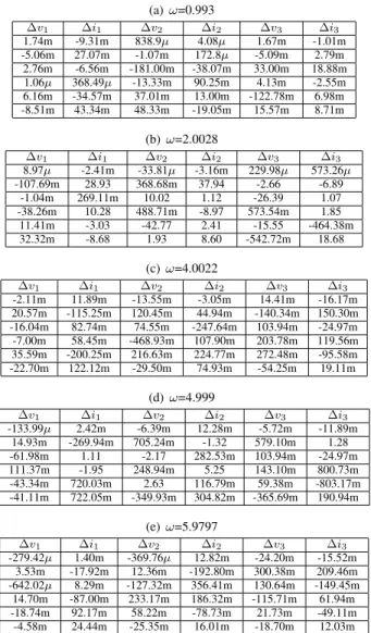
In this study, we derive the variational circuit which corre- sponds to the variational equation and perform the transient analysis of Spice just for one period in order to obtain the components of Φ(T ). We should repeat the transient analysis by giving different initial conditions to obtain all the components numerically. However, the number of the repeat is at most the same as the number of the state variables of the circuit. Further, it should be mentioned that we do not have to change the structure of the variational circuit even when the voltages of the regular periodic solution are changed.

III. I LLUSTRATIVE EXAMPLE

As an illustrative example, we assess the stability with the circuit in Fig. 3. The circuit parameters in Fig. 3 are set as α = β = 1, R 1 = R 2 = R 3 = 0.1, L 1 = 0.4167, L 2 = 0.2618, L 3 = 1.058, C 1 = 0.1, C 2 = 0.3429 and C 3 = 0.439.

- 153 -

C 3

i G

v G

+

−

Fig. 3. Cauer oscillator.

The circuit equation can be written as

 

 

 

 

 

 

 

 C ₁ dv ₁

dt + i ₁ = αv ₁ − βv ₁ ³ i 1 = i 2 + C 2

dv 2

dt i 2 = i 3 + C 3

dv 3

dt

. (16)

If we write the variables as periodic solutions with small

variations; {

i _k = i _k0 + ∆i _k

v _k = v _k0 + ∆v _k (17)

We obtain the following variational equations as

 

 

 

 

 

 

 

 C 1

dv ₁₀

dt + ∆i 1 = α∆v 1 − 3βv 10 2 ∆v 1

∆i ₁ = ∆i ₂ + C ₂ ∆dv 2

dt

∆i 2 = ∆i 3 + C 3

∆dv 3

dt

, (18)

where we neglect higher-order small terms. From these equa- tions, we can make the variational circuit of Fig. 3 as shown in Fig. 4.

C

3

v

1

∆

1 2 10

) 3 ( α − β v ∆ v

v

2

∆ ∆ v

₃

Fig. 4. Variational circuit of Fig. 3.

In Fig. 4, v 10 is a steady periodic solution and are calculated as

v 10 = V c cos ωt + V s sin ωt, (19) where V c and V s are given by the sine-cosine circuit obtained from the circuit in Fig. 3.

IV. S IMULATION RESULTS

Fig. 5. Result of transient analysis in Fig.4.

Figure 5 is the time-response obtained by solving the circuit in Fig. 3 with HB method combining with Newton homotopy method. We found 5 equilibrium points, where ρ (=V(RO)) satisfying ρ = 1. We show the solutions in Table I.

TABLE I

E

IGENVALUES OBTAINED BY CONVENTIONAL METHOD

time [sec] 1.5728 20.26 32.72 34.723 36.694 V(Omega) 0.993 2.003 4.002 4.999 5.9797 V(VC1) 1.211 9.446 1.216 2.346 1.1918 V(IL1) 0.1563 65.945 0.499 3.339 0.716 V(VC2) 1.1520 54.84 0.416 6.410 0.598 V(IL2) 0.520 28.398 1.03 7.853 0.513 V(VC3) 1.009 69.43 0.677 3.9160 0.208 V(IL3) 0.956 32.727 0.160 0.740 0.033

We give the obtained value to the circuit of Fig. 4 as initial condition. The state of initial condition are given as follows;

(∆v ₁₀ , ∆i ₁₀ , ∆v ₂₀ , ∆i ₂₀ , ∆v ₃₀ , ∆i ₃₀ ) (20)

=

 

 

 

 

 



 

 

 

 

 

(V(VC1), 0, 0, 0, 0, 0) (0,V(IL1), 0, 0, 0, 0) (0, 0,V(VC2), 0, 0, 0) (0, 0, 0,V(IL2), 0, 0) (0, 0, 0, 0,V(VC3), 0) (0, 0, 0, 0, 0,V(IL3))

. (21)

We perform the transient analysis with the circuit in Fig. 4 just for one period and obtain the components of Φ(T ) as the values of the state variables of the variational circuit. We show Φ(T) for the 5 cases in Table II. Table III shows eigenvalues of Φ(T ) for 5 cases, which calculated by MATLAB. We can see that the point ω = 0.993, ω = 4.0022 and ω = 5.9797 are stable, because all of eigenvalues satisfy | λ | < 1. However, for the other two points, ω = 2.0028 and ω = 4.999, the solutions are unstable, because some eigenvalues do not satisfy | λ | < 1.

These results agree with the results obtained in [4]. Namely, we can say that our algorithm gives the correct results.

- 154 -

TABLE II

T

HE VALUES AFTER ONE PERIOD

Φ(T )

(a) ω=0.993

∆v

1

∆i

1

∆v

2

∆i

2

∆v

3

∆i

3

1.74m -9.31m 838.9µ 4.08µ 1.67m -1.01m -5.06m 27.07m -1.07m 172.8µ -5.09m 2.79m 2.76m -6.56m -181.00m -38.07m 33.00m 18.88m 1.06µ 368.49µ -13.33m 90.25m 4.13m -2.55m 6.16m -34.57m 37.01m 13.00m -122.78m 6.98m -8.51m 43.34m 48.33m -19.05m 15.57m 8.71m

(b) ω=2.0028

∆v

1

∆i

1

∆v

2

∆i

2

∆v

3

∆i

3

8.97µ -2.41m -33.81µ -3.16m 229.98µ 573.26µ -107.69m 28.93 368.68m 37.94 -2.66 -6.89

-1.04m 269.11m 10.02 1.12 -26.39 1.07 -38.26m 10.28 488.71m -8.97 573.54m 1.85 11.41m -3.03 -42.77 2.41 -15.55 -464.38m

32.32m -8.68 1.93 8.60 -542.72m 18.68

(c) ω=4.0022

∆v

1

∆i

1

∆v

2

∆i

2

∆v

3

∆i

3

-2.11m 11.89m -13.55m -3.05m 14.41m -16.17m 20.57m -115.25m 120.45m 44.94m -140.34m 150.30m -16.04m 82.74m 74.55m -247.64m 103.94m -24.97m -7.00m 58.45m -468.93m 107.90m 203.78m 119.56m 35.59m -200.25m 216.63m 224.77m 272.48m -95.58m -22.70m 122.12m -29.50m 74.93m -54.25m 19.11m

(d) ω=4.999

∆v

1

∆i

1

∆v

2

∆i

2

∆v

3

∆i

3

-133.99µ 2.42m -6.39m 12.28m -5.72m -11.89m

14.93m -269.94m 705.24m -1.32 579.10m 1.28 -61.98m 1.11 -2.17 282.53m 103.94m -24.97m 111.37m -1.95 248.94m 5.25 143.10m 800.73m -43.34m 720.03m 2.63 116.79m 59.38m -803.17m -41.11m 722.05m -349.93m 304.82m -365.69m 190.94m

(e) ω=5.9797

∆v

1

∆i

1

∆v

2

∆i

2

∆v

3

∆i

3

-279.42µ 1.40m -369.76µ 12.82m -24.20m -15.52m

3.53m -17.92m 12.36m -192.80m 300.38m 209.46m -642.02µ 8.29m -127.32m 356.41m 130.64m -149.45m 14.70m -87.00m 233.17m 186.32m -115.71m 61.94m -18.74m 92.17m 58.22m -78.73m 21.73m -49.11m -4.58m 24.44m -25.35m 16.01m -18.70m 12.03m

V. C ONCLUSION

We proposed the SPICE-oriented algorithm to assess the stability of periodic solutions for oscillator. We obtained periodic solutions by using harmonic balance method and Newton homotopy method. We assessed the stability based on the Floquet theory. In detail, we analyzed the Cauer oscil- lator for 5 different frequencies which gives both stable and unstable solutions. Our results agree well with the previously obtained results. For the next step of our research, we need to work on assessment of stability of oscillator having complex characteristics.

R EFERENCES

[1] H. Kataoka, Y. Yamagami and Y. Nishio, “SPICE-Oriented Algorithm for Assessment of Stability for Periodic Solutions,” Proc. of NOLTA’10, pp.374-377, 2010.

[2] Y. Inoue, “DC Analysis of Nonlinear Circuits Using Solution-Tracing Circuits,” Trans. IEICE, vol.J74-A, pp.1647-1655, 1991.

TABLE III E

IGENVALUES OF

Φ(T ).

ω 0.993 2.003 4.002 4.999 5.980 λ

1

− 0.202 − 38.947 -0.411 5.670 0.402 λ

2

− 0.112 0 0.467 -4.154 -0.359 λ

3

0.093 − 18.424 0.365 -1.717 0.181 λ

4

0.034 18.120 -0.186 0 -0.004

λ

5

0 39.230 0 2.889 0.050

λ

6

0.101 33.133 0.122 0.885 -0.196

[3] A. Ushida, Y. Yamagami, I. Kinouchi, Y. Nishio and Y. Inoue, “An Efficient Algorithm for Finding Multiple DC Solutions Based on the SPICE-Oriented Newton Homotopy Method,” IEEE Trans. Computer- Aided Design of Integrated Circuits Syst., vol.21, no.3, pp.337-348, Mar.

2002.

[4] Y. Yamagami, Y. Nishio and A. Ushida, “Analysis of Reactance oscillators Having Multi-Mode Oscillations,” IEICE Trans. Fundamentals., vol.E89- A, no.3 Mar. 2006.

[5] J. Kawata, Y. Taniguchi, M. Oda, Y. Yamagami, Y. Nishio and A. Ushida,

“SPICE-Oriented Frequency-Domain Analysis of Nonlinear Electronic Circuits,” IEICE Trans. Fundamentals, vol.E90-A, no.2, Feb. 2007.

[6] P. Wambacq and W. Sansen, Distortion Analysis of Analog Integrated Circuits, Kluwer Academic Publishers, 1979.

[7] D.O. Pederson and K. Mayaram, Analog Integrated Circuits for Commu- nication, Kluwer Academic Publishers, 1991.

[8] A.H. Nayfeh and D.T. Mook, Nonlinear Oscillations, Wiley-Inter Science, 1998.

[9] E. Ikeno and A. Ushida, “The Arc-Length Method for the Computation of Characteristic Curves,” IEEE Trans. Circuits Syst., vol.23, pp.181-183, 1976.

[10] F.L. Traversa, F. Bonani and S.D. Guerrieri, “A Frequency-Domain Approach to the Analysis of Stability and Bifurcations in Nonlinear Systems Described by Differential-Algebraic Equations,” Int. J. Circuit Theory and Appl., vol.36, pp.421-439, 2008.

- 155 -