Research of Two Coupled Maps with Intermittency Chaos
Yuki Fujisawa, Yoko Uwate and Yoshifumi Nishio
Dept. Electrical and Electronic Eng.,Tokushima University Email:
{fujisawa, uwate, nishio
}@ee.tokushima-u.ac.jp Abstract—Generally, complex dynamical phenomena
can be observed in networks formed by many elements with nonlinearity. Coupled Map Lattice has proposed by Kaneko, to represent the complex high-dimensional dy- namics, for example biological systems, networks in DNA, and neural networks. In this study, we investigate the in- fluence of the delay in two coupled cubic maps with in- termittency chaos. Moreover, the relation between average length of laminar part and the combination of delay is in- vestigated.
1. Introduction
Generally, complex dynamical phenomena can be ob- served in networks formed by many elements with non- linearity. Coupled Map Lattice (CML) has proposed by Kaneko [1]-[4], to represent the complex high-dimensional dynamics, for example biological systems, networks in DNA, economic activities and neural networks. Further- more, we focus on intermittency chaos and delay. The delay naturally occurs from information transmission and processing speeds in the realistic networks[5]. In Ref.[5], the study investigated the synchronization states of the cou- pled logistic maps with the delay. As a result, the synchro- nization state of coupled chaotic maps are induced by the delay. Therefore, the studies considered the delay in cou- pled chaotic maps are investigated actively. In addition, in- termittency chaos has stability and mobility and gains good result for information processing. We consider that inter- mittency chaos is related to various phenomena[6][7], e.g, information processing of the brain. In order to make clear the mechanism of such phenomena in various fields, un- veiling the roles of intermittency chaos is very important.
In this study, we focus on the influence of the delay in two coupled cubic maps with intermittency chaos
1. When we set a control parameter of two cubic maps to generate intermittency chaos near the six periodic window, various synchronization states are confirmed in laminar part. More- over, the relation between average length of laminar part and combination of the delay is investigated.
1This study revised NCSP’16[8]
2. Two coupled cubic maps
A cubic map is expressed as follows:
f
(x)
=ax3+x(1+a),(1) where
arepresents a control parameter.
a
Figure 1: The bifurcation diagram of cubic map.
a
f(x)
a
Figure 2: The boundary of six periodic window.
Figure 1 shows the bifurcation diagram of cubic map.
This figure shows period-doubling bifurcations and peri- odic windows (near
a =-3.69, -3.83). We focus on the boundary of periodic windows in the bifurcation diagram of cubic map. At the boundary of six periodic window intermittency chaos is observed in Fig. 2. Laminar rep- resents the periodic state and burst represents the chaotic state. We define
a =-3.69964153 representing the co- existence of laminar and burst in here. Figure 3 shows
- 44 -
IEEE Workshop on Nonlinear Circuit Networks December 9-10, 2016
the time series of cubic map with intermittency chaos (a
=
-3.69964153). This figure shows intermittency chaos is switching between laminar and burst. Furthermore, in the case of
a=-3.69964153, intermittency chaos including six periodic laminars are observed.
i
f(x)
Figure 3: Time series of cubic map with intermittency chaos (a
=-3.69964153).
In this study, we consider two coupled cubic maps with the delay. The coupling system is expressed as follows:
{ x(1,i+1)=
(1
−g)f(x
(1,i))
+g f(x
(2,i−τ1))
x(2,i+1)=
(1
−g)f(x
(2,i))
+g f(x
(1,i−τ2))
,(2) where
grepresents the coupling strength,
τ1and
τ2repre- sents the delay between the maps.
3. Simulation Results
3.1. Average length of laminar part
In this study, the initial conditions and the parameters of two cubic maps are fixed with
x(1,0)=0.1,
x(2,0)=-0.2,
g=
0.0000001, 0.00001, respectively. The iteration time is fixed with
i=200000. And range of the delay is
τ1and
τ2 =0, 1,
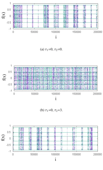
· · ·, 12. Figures 4 and 5 show the time series of coupled cubic maps with the delay. Laminar during the iteration time is longer than the other, e.g, Figs. 4 (a), (c) and Figs. 5 (a), (c). The others almost aren’t observed the laminar part, e.g, Figs. 4 (b) and Figs. 5 (b). As a result, increasing the value of the coupling strength, the di
fference of laminar and burst can be clearly seen.
Next, we investigate the length of laminar part in coupled cubic maps with the delay. In order to investigate quantita- tive average length of laminar part, we define laminar part by
|x− ±0
.1895 or
±0
.4865 or
±0
.8873
|<0
.0001. Fig- ures 6 and 7 show the average length of laminar part during the iteration time. From Fig. 6, if the case of non-delay (
τ1=0,
τ2 =0), average length of laminar part is 1547. In the case of
τ1+τ2 =6n (n
=1,2,3,4), the average length of laminar parts are longer. The others has become less than 200. Among the
τ1+τ2=6n, than when the case of non-delay, combinations of
τ1 +τ2 =6n that the synchro- nization state is longer than non-delay is confirmed thir- teen locations. From Fig. 7, if the case of non-delay (
τ1=
0,
τ2 =0), the average length of laminar part is 10366, because the density of burst part is increased when the cou- pling strength is high. In the case of
τ1 + τ2 =6n, the average length of laminar parts are longer than Fig. 6. The others has become less than 30. Among the
τ1+τ2=6n, than when the case of non-delay, combinations of
τ1 +τ2=
6n that the synchronization state is longer than non-delay is confirmed six locations.
f(x)
i
(a)τ1=0,τ2=0.
i
f(x)
(b)τ1=0,τ2=3.
f(x)
i
(c)τ1=1,τ2=5.
Figure 4: Time series of coupled cubic maps (g
=0.0000001).
- 45 -
f(x)
i
(a)τ1=0,τ2=0.
f(x)
i
f(x)
i
(b)τ1=0,τ2=3.
f(x)
i
(c)τ1=1,τ2=5.
Figure 5: Time series of coupled cubic maps (g
=0.00001).
Figure 6: Average length of laminar part (g
=0.0000001).
Figure 7: Average length of laminar part (g
=0.00001).
3.2. Synchronization Pattern
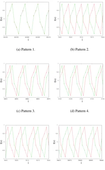
Laminar part is composed of one of the six synchroniza- tion states. There is all the patterns within each the time series in Figs. 8. For example, Figs. 8(a) show in-phase synchronous and Figs. 8(b) show anti-phase synchronous.
It don’t have variation in the synchronization state until switched to burst part. We investigate whether the syn- chronization state that constitutes the laminar part there is variation by the combination of the delay. In this study, we focus on the synchronization states of each of the length of laminar part is more than 3,000. All synchronization states of this laminar part in the time series is the same synchro- nization pattern. When the case of non-delay, we search in-phase synchronous laminar parts are only. But, Fig. 9 shows variation of the synchronization states in the combi- nation of
τ1+τ2=6n (n
=1,2,3,4).
In addition, we searched the synchronization state con- sists of in-phase synchronous to anti-phase synchronous, it returns to the in-phase synchronous regularity when we set
τ1+τ2=6n. For example, when we set
τ1+τ2=6n, the synchronization state change Figs. 8(a), (c), (e), (b), (f), (d), (a). We haven’t searched variation to the coupling strength in the synchronization states.
4. Conclusions
In this study, we have investigated the influence of the delay in two coupled cubic maps with intermittency chaos.
First, we observed the time series of coupled cubic maps with the delay.
Next, we investigated the length of laminar part in cou- pled cubic maps with the delay. The average length of lam- inar part is longer than others when the delay is set to
τ1+τ2 =
6n (n
=1,2,3,4). As a result, we could consider two maps with six periodic solution easily to become to the synchronization states when
τ1+τ2=6n.
Finally, we focus on the synchronization pattern of each of the length of laminar part is more than 3,000 when
τ1+ τ2=6n. We searched the synchronization state consists of in-phase synchronous to anti-phase synchronous, it returns
- 46 -
to the in-phase synchronous regularity in the combination of
τ1+τ2=6n .
i
f(x)
(a) Pattern 1.
i
f(x)
(b) Pattern 2.
i
f(x)
(c) Pattern 3.
i
f(x)
(d) Pattern 4.
i
f(x)
(e) Pattern 5.
i
f(x)
(f) Pattern 6.