6 Bayesian Estimation — Examples

6 Bayesian Estimation — Examples

6.1 Heteroscedasticity Model

In Section 6.1, Tanizaki and Zhang (2001) is re-computed using the random number generators.

Here, we show how to use Bayesian approach in the multiplicative heteroscedastic- ity model discussed by Harvey (1976).

The Gibbs sampler and the Metropolis-Hastings (MH) algorithm are applied to the multiplicative heteroscedasticity model, where some sampling densities are consid-

ered in the MH algorithm.

We carry out Monte Carlo study to examine the properties of the estimates via Bayesian approach and the traditional counterparts such as the modified two-step estimator (M2SE) and the maximum likelihood estimator (MLE).

The results of Monte Carlo study show that the sampling density chosen here is suit- able, and Bayesian approach shows better performance than the traditional counter- parts in the criterion of the root mean square error (RMSE) and the interquartile range (IR).

6.1.1 Introduction

For the heteroscedasticity model, we have to estimate both the regression coeffi- cients and the heteroscedasticity parameters.

In the literature of heteroscedasticity, traditional estimation techniques include the two-step estimator (2SE) and the maximum likelihood estimator (MLE).

Harvey (1976) showed that the 2SE has an inconsistent element in the heteroscedas- ticity parameters and furthermore derived the consistent estimator based on the 2SE, which is called the modified two-step estimator (M2SE).

These traditional estimators are also examined in Amemiya (1985), Judge, Hill,

Griffiths and Lee (1980) and Greene (1997).

Ohtani (1982) derived the Bayesian estimator (BE) for a heteroscedasticity linear model.

Using a Monte Carlo experiment, Ohtani (1982) found that among the Bayesian estimator (BE) and some traditional estimators, the Bayesian estimator (BE) shows the best properties in the mean square error (MSE) criterion.

Because Ohtani (1982) obtained the Bayesian estimator by numerical integration, it is not easy to extend to the multi-dimensional cases of both the regression coeffi- cient and the heteroscedasticity parameter.

Recently, Boscardin and Gelman (1996) developed a Bayesian approach in which a Gibbs sampler and the Metropolis-Hastings (MH) algorithm are used to estimate the parameters of heteroscedasticity in the linear model.

They argued that through this kind of Bayesian approach, we can average over our uncertainty in the model parameters instead of using a point estimate via the traditional estimation techniques.

Their modeling for the heteroscedasticity, however, is very simple and limited.

Their choice of the heteroscedasticity is V(yi)= σ²w^−θ_i , where wiare known “weights”

for the problem andθis an unknown parameter.

In addition, they took only one candidate for the sampling density used in the MH algorithm and compared it with 2SE.

In Section 6.1, we also consider Harvey’s (1976) model of multiplicative heteroscedas- ticity.

This modeling is very flexible, general, and includes most of the useful formulations for heteroscedasticity as special cases.

The Bayesian approach discussed by Ohtani (1982) and Boscardin and Gelman (1996) can be extended to the multi-dimensional and more complicated cases, using the model introduced here.

The Bayesian approach discussed here includes the MH within Gibbs algorithm, where through Monte Carlo studies we examine two kinds of candidates for the sampling density in the MH algorithm and compare the Bayesian approach with the two traditional estimators, i.e., M2SE and MLE, in the criterion of the root mean square error (RMSE) and the interquartile range (IR).

We obtain the results that the Bayesian estimator significantly has smaller RMSE and IR than M2SE and MLE at least for the heteroscedasticity parameters.

Thus, the results of the Monte Carlo study show that the Bayesian approach per- forms better than the traditional estimators.

6.1.2 Multiplicative Heteroscedasticity Regression Model

The multiplicative heteroscedasticity model discussed by Harvey (1976) can be shown as follows:

yt =Xtβ+ut, ut ∼ N(0, σ²t), (7)

σ²t = σ²exp(qtα), (8)

for t = 1,2,· · ·,n, where y_t is the tth observation, X_t and q_t are the tth 1×k and 1×(J−1) vectors of explanatory variables, respectively.

βandαare vectors of unknown parameters.

The model given by equations (7) and (8) includes several special cases such as the model in Boscardin and Gelman (1996), in which qt = log wtandθ=−α.

As shown in Greene (1997), there is a useful simplification of the formulation.

Let zt =(1,qt) andγ=(logσ², α⁰)⁰, where zt andγdenote 1×J and J×1 vectors.

Then, we can simply rewrite equation (8) as:

σ²t =exp(ztγ). (9)

Note that exp(γ1) providesσ², whereγ1denotes the first element ofγ. As for the variance of u_t, hereafter we use (9), rather than (8).

The generalized least squares (GLS) estimator ofβ, denoted by ˆβGLS, is given by:

βˆGLS =(∑ⁿ

t=1

exp(−z_tγ)X_t⁰X_t)₋1∑n t=1

exp(−z_tγ)X_t⁰y_t, (10) where ˆβGLS depends onγ, which is the unknown parameter vector.

To obtain the feasible GLS estimator, we need to replace γ by its consistent esti- mate.

We have two traditional consistent estimators ofγ, i.e., M2SE and MLE, which are briefly described as follows.

Modified Two-Step Estimator (M2SE): First, define the ordinary least squares (OLS) residual by et = yt − XtβˆOLS, where ˆβOLS represents the OLS estimator, i.e., βˆOLS = (∑n

t=1X_t⁰X_t)⁻¹∑n t=1X_t⁰y_t.

For 2SE ofγ, we may form the following regression:

log e²_t = z_tγ+v_t.

The OLS estimator ofγapplied to the above equation leads to the 2SE ofγ, because e_t is obtained by OLS in the first step.

Thus, the OLS estimator ofγgives us 2SE, denoted by ˆγ2S E, which is given by:

γˆ2S E = (

∑n t=1

z⁰_tz_t)⁻¹

∑n t=1

z⁰_tlog e²_t.

A problem with this estimator is that v_t, t = 1,2,· · ·,n, have non-zero means and are heteroscedastic.

If e_t converges in distribution to u_t, the v_t will be asymptotically independent with mean E(v_t) = −1.2704 and variance V(v_t) = 4.9348, which are shown in Harvey (1976).

Then, we have the following mean and variance of ˆγ2S E: E( ˆγ2S E)=γ−1.2704(

∑n t=1

z⁰_tzt)⁻¹

∑n t=1

z⁰_t, (11)

V( ˆγ2S E)=4.9348(

∑n t=1

z⁰_tzt)⁻¹.

For the second term in equation (11), the first element is equal to−1.2704 and the remaining elements are zero, which can be obtained by simple calculation.

Therefore, the first element of ˆγ2S E is biased but the remaining elements are still unbiased.

γ γ γ

which is given by:

γˆM2S E =γˆ2S E +1.2704(

∑n t=1

z⁰_tz_t)⁻¹

∑n t=1

z⁰_t. LetΣM2S E be the variance of ˆγM2S E.

Then,ΣM2S E is represented by:

ΣM2S E ≡V( ˆγM2S E)=V( ˆγ2S E)= 4.9348(

∑n t=1

z⁰_tzt)⁻¹.

The first element of ˆγ2S E and ˆγM2S E corresponds to the estimate ofσ², which value does not influence ˆβGLS.

Since the remaining elements of ˆγ2S E are equal to those of ˆγM2S E, ˆβ2S E is equivalent to ˆβM2S E, where ˆβ2S E and ˆβM2S E denote 2SE and M2SE ofβ, respectively.

Note that ˆβ2S E and ˆβM2S E can be obtained by substituting ˆγ2S E and ˆγM2S E intoγin (10).

Maximum Likelihood Estimator (MLE): The density of Y_n = (y₁, y₂, · · ·, y_n) based on (7) and (9) is:

f (Y_n|β, γ)∝ exp



−1 2

∑n t=1

(exp(−z_tγ)(y_t −X_tβ)²+z_tγ)



, (12) which is maximized with respect toβandγ, using the method of scoring.

That is, given values forβ^{( j)} andγ^{( j)}, the method of scoring is implemented by the following iterative procedure:

β^{( j)} =(∑ⁿ

t=1

exp(−ztγ^{( j−1)})X_t⁰Xt

)₋₁∑ⁿ

t=1

exp(−ztγ^{( j−1)})X⁰_tyt, γ^{( j)} =γ^{( j−1)}+2(

∑n t=1

z⁰_tzt)⁻¹1 2

∑n t=1

z⁰_t(

exp(−ztγ^{( j−1)})e²_t −1) , for j=1,2,· · ·,where e_t = y_t−X_tβ^{( j−1)}.

The starting value for the above iteration may be taken as (β⁽⁰⁾, γ⁽⁰⁾)= ( ˆβOLS,γˆ2S E), ( ˆβ2S E,γˆ2S E) or ( ˆβM2S E,γˆM2S E).

Letθ =(β, γ).

The limit of θ^{( j)} = (β^{( j)}, γ^{( j)}) gives us the MLE of θ, which is denoted by ˆθMLE = ( ˆβMLE, ˆγMLE).

Based on the information matrix, the asymptotic covariance matrix of ˆθMLE is repre- sented by:

V(ˆθMLE)= (

−E

(∂²log f (Y_n|θ)

∂θ∂θ⁰

))₋1

= ( (∑ⁿ

t=1exp(−ztγ)X_t⁰Xt

)₋₁

0

0 2(∑n

t=1z⁰_tz_t)⁻¹ )

. (13)

Thus, from (13), asymptotically there is no correlation between ˆβMLE and ˆγMLE, and

γ Σ ≡ γ =

2(∑n

t=1z⁰_tz_t)⁻¹, which implies that ˆγM2S E is asymptotically inefficient becauseΣM2S E − ΣMLE is positive definite.

Remember that the variance of ˆγM2S E is given by: V( ˆγM2S E)= 4.9348(∑n

t=1z⁰_tz_t)⁻¹.

6.1.3 Bayesian Estimation

We assume that the prior distributions of the parametersβandγare noninformative, which are represented by:

f_β(β)=constant, f_γ(γ)=constant. (14)

Combining the prior distributions (14) and the likelihood function (12), the poste- rior distribution f_βγ(β, γ|y) is obtained as follows:

f_βγ(β, γ|Y_n)∝ exp



−1 2

∑n t=1

(exp(−z_tγ)(y_t−X_tβ)²+z_tγ)



. The posterior means ofβandγare not operationally obtained.

Therefore, by generating random draws ofβandγfrom the posterior density f_βγ(β, γ|Yn), we consider evaluating the mathematical expectations as the arithmetic averages based on the random draws.

Now we utilize the Gibbs sampler, which has been introduced in Section 5.7.5, to

β γ

Then, from the posterior density f_βγ(β, γ|Y_n), we can derive the following two con- ditional densities:

f_γ|β(γ|β,Y_n)∝exp



−1 2

∑n t=1

(exp(−z_tγ)(y_t −X_tβ)²+z_tγ)



, (15)

f_β|γ(β|γ,Y_n)=N(B₁,H₁), (16)

where

H₁⁻¹ =

∑n t=1

exp(−z_tγ)X_t⁰X_t, B₁ = H₁

∑n t=1

exp(−z_tγ)X_t⁰y_t.

Sampling from (16) is simple since it is a k-variate normal distribution with mean B1 and variance H1.

However, since the J-variate distribution (15) does not take the form of any standard density, it is not easy to sample from (15).

In this case, the MH algorithm discussed in Section 5.7.3 can be used within the Gibbs sampler.

See Tierney (1994) and Chib and Greeberg (1995) for a general discussion.

Letγi−1 be the (i−1)th random draw ofγ andγ^∗be a candidate of the ith random draw ofγ.

The MH algorithm utilizes another appropriate distribution function f_∗(γ|γi), which is called the sampling density or the proposal density.

Let us define the acceptance rateω(γi−1, γ^∗) as:

ω(γi−1, γ^∗)= min

( f_γ|β(γ^∗|βi−1,Y_n)/f_∗(γ^∗|γi−1) f_γ|β(γi−1|βi−1,Y_n)/f_∗(γi−1|γ^∗), 1

) .

The sampling procedure based on the MH algorithm within Gibbs sampling is as follows:

(i) Set the initial valueβ₋M, which may be taken as ˆβM2S E or ˆβMLE.

(ii) Givenβi−1, generate a random draw ofγ, denoted byγi, from the conditional density f_γ|β(γ|βi−1,Y_n), where the MH algorithm is utilized for random number generation because it is not easy to generate random draws ofγfrom (15).

The Metropolis-Hastings algorithm is implemented as follows:

(a) Givenγi−1, generate a random drawγ^∗from f_∗(·|γi−1) and compute the acceptance rateω(γi−1, γ^∗).

We will discuss later about the sampling density f_∗(γ|γi−1).

(b) Setγi = γ^∗with probabilityω(γi−1, γ^∗) andγi = γi−1otherwise,

(iii) Givenγi, generate a random draw ofβ, denoted by βi, from the conditional density f_β|γ(β|γi,Yn), which isβ|γi,Yn ∼ N(B1,H1) as shown in (16).

(iv) Repeat (ii) and (iii) for i=−M+1,−M+2,· · ·,N.

Note that the iteration of Steps (ii) and (iii) corresponds to the Gibbs sampler, which iteration yields random draws ofβandγ from the joint density f_βγ(β, γ|Yn) when i is large enough.

It is well known that convergence of the Gibbs sampler is slow when β is highly correlated withγ.

That is, a large number of random draws have to be generated in this case.

Therefore, depending on the underlying joint density, we have the case where the Gibbs sampler does not work at all.

For example, see Chib and Greenberg (1995) for convergence of the Gibbs sampler.

In the model represented by (7) and (8), however, there is asymptotically no corre- lation between ˆβMLE and ˆγMLE, as shown in (13).

It might be expected that correlation between ˆβMLE and ˆγMLE is not too high even in the small sample.

Therefore, it might be appropriate to consider that the Gibbs sampler works well in this model.

In Step (ii), the sampling density f_∗(γ|γi−1) is utilized.

We consider the multivariate normal density function for the sampling distribution, which is discussed as follows.

Choice of the Sampling Density in Step (ii): Several generic choices of the sam- pling density are discussed by Tierney (1994) and Chib and Greenberg (1995).

Here, we take f_∗(γ|γi−1) = f_∗(γ) as the sampling density, which is called the inde- pendence chain because the sampling density is not a function ofγi−1.

We consider taking the multivariate normal sampling density in the independence MH algorithm, because of its simplicity.

Therefore, f_∗(γ) is taken as follows:

f_∗(γ)=N(γ⁺,c²Σ⁺), (17) which represents the J-variate normal distribution with meanγ⁺and variance c²Σ⁺.

The tuning parameter c is introduced into the sampling density (17).

We have mentioned that for the independence chain (Sampling Density I) the sam- pling density with the variance which gives us the maximum acceptance probability is not necessarily the best choice.

From some Monte Carlo experiments, we have obtained the result that the sampling density with the 1.5 – 2.5 times larger standard error is better than that with the standard error which maximizes the acceptance probability.

Therefore, c = 2 is taken in the next section, and it is the larger value than the c which gives us the maximum acceptance probability.

This detail discussion is given in Section 6.1.4.

Thus, the sampling density ofγis normally distributed with meanγ⁺and variance c²Σ⁺.

As for (γ⁺,Σ⁺), in the next section we choose one of ( ˆγM2S E,ΣM2S E) and ( ˆγMLE,ΣMLE) from the criterion of the acceptance rate.

As shown in Section 2, both of the two estimators ˆγM2S E and ˆγMLE are consistent estimates ofγ.

Therefore, it might be very plausible to consider that the sampling density is dis- tributed around the consistent estimates.

Bayesian Estimator: From the convergence theory of the Gibbs sampler and the MH algorithm, as i goes to infinity we can regardγi andβi as random draws from the target density f_βγ(β, γ|Y_n).

Let M be a sufficiently large number. γi andβi for i = 1,2,· · ·,N are taken as the random draws from the posterior density f_βγ(β, γ|Y_n).

Therefore, the Bayesian estimators ˆγBZZ and ˆβBZZ are given by:

γˆBZZ = 1 N

∑N i=1

γi, βˆBZZ = 1 N

∑N i=1

βi,

where we read the subscript BZZ as the Bayesian estimator which uses the multi-

γ Σ

or MLE.

We consider two kinds of candidates of the sampling density for the Bayesian esti- mator, which are denoted by BM2SE and BMLE.

Thus, in Section 6.1.4, we compare the two Bayesian estimators (i.e, BM2SE and BMLE) with the two traditional estimators (i.e., M2SE and MLE).

6.1.4 Monte Carlo Study

Setup of the Model: In the Monte Carlo study, we consider using the artificially simulated data, in which the true data generating process (DGP) is presented in

Judge, Hill, Griffiths and Lee (1980, p.156).

The DGP is defined as:

y_t =β1+β2x_2,t+β3x_3,t +u_t, (18) where u_t, t=1,2,· · ·,n, are normally and independently distributed with E(u_t)= 0, E(u²_t)=σ²t and,

σ²t =exp(γ1+γ2x_2,t), for t = 1,2,· · ·,n. (19) As it is discussed in Judge, Hill, Griffiths and Lee (1980), the parameter values are

β , β , β γ , γ = , , ,− , .

From (18) and (19), Judge, Hill, Griffiths and Lee (1980, pp.160 – 165) generated one hundred samples of y with n=20.

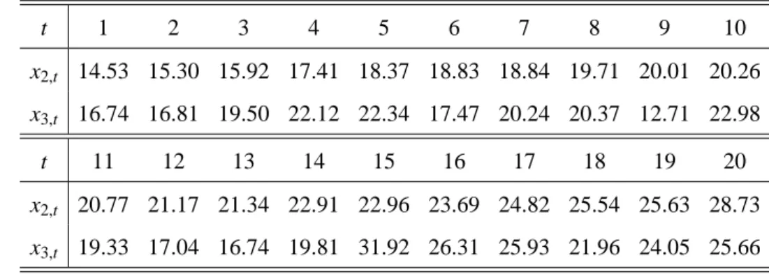
In the Monte Carlo study, we utilize x_2,t and x_3,t given in Judge, Hill, Griffiths and Lee (1980, pp.156), which is shown in Table 1, and generate G samples of yt given the X_t for t= 1,2,· · ·,n.

That is, we perform G simulation runs for each estimator, where G =10⁴is taken.

The simulation procedure is as follows:

(i) Given γ and x2,t for t = 1,2,· · ·,n, generate random numbers of ut for t = 1,2,· · ·,n, based on the assumptions: u_t ∼ N(0, σ²_t), where (γ1, γ2) =

Table 1: The Exogenous Variables x_1,t and x_2,t

t 1 2 3 4 5 6 7 8 9 10

x2,t 14.53 15.30 15.92 17.41 18.37 18.83 18.84 19.71 20.01 20.26 x_3,t 16.74 16.81 19.50 22.12 22.34 17.47 20.24 20.37 12.71 22.98

t 11 12 13 14 15 16 17 18 19 20

x_2,t 20.77 21.17 21.34 22.91 22.96 23.69 24.82 25.54 25.63 28.73 x3,t 19.33 17.04 16.74 19.81 31.92 26.31 25.93 21.96 24.05 25.66

(−2,0.25) andσ²_t =exp(γ1+γ2x_2,t) are taken.

(ii) Given β, (x_2,t,x_3,t) and u_t for t = 1,2,· · ·,n, we obtain a set of data y_t, t = 1,2,· · ·,n, from equation (18), where (β1, β2, β3)=(10,1,1) is assumed.

(iii) Given (y_t,X_t) for t = 1,2,· · ·,n, perform M2SE, MLE, BM2SE and BMLE discussed in Sections 6.1.2 and 6.1.3 in order to obtain the estimates ofθ = (β, γ), denoted by ˆθ.

Note that ˆθtakes ˆθM2S E, ˆθMLE, ˆθBM2S E and ˆθBMLE.

(iv) Repeat (i) – (iii) G times, where G=10⁴is taken as mentioned above.

(v) From G estimates ofθ, compute the arithmetic average (AVE), the root mean

square error (RMSE), the first quartile (25%), the median (50%), the third quartile (75%) and the interquartile range (IR) for each estimator.

AVE and RMSE are obtained as follows:

AVE = 1 G

∑G g=1

θˆ^(g)_j , RMSE= (1 G

∑G g=1

(ˆθ^(g)_j −θj)²)_1/2 ,

for j = 1,2,· · ·,5, whereθj denotes the jth element of θand ˆθ^(g)_j represents the j-element of ˆθin the gth simulation run.

As mentioned above, ˆθdenotes the estimate of θ, where ˆθ takes ˆθM2S E, ˆθMLE, θˆ and ˆθ .

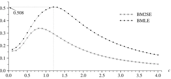
Figure 2: Acceptance Rates in Average: M = 5000 and N =10⁴

0.0 0.1 0.2 0.3 0.4 0.5

0.0 0.5 1.0 1.5 2.0 2.5 3.0 3.5 4.0

c

× × ×

×

×

× × × × × ×

× ×

× ×

× ×

× × × ×

× × ×

× × × ×

× × × × × × × × × × × ×

• • •

•

•

•

•

• • • • • • •

• •

• •

• •

• •

• •

• • •

• • • •

• • •

• • • • • •

× × × × BM2SE

• • • • BMLE HH

Y 0.508

Choice of (γ⁺,Σ⁺) and c: For the Bayesian approach, depending on (γ⁺,Σ⁺) we have BM2SE and BMLE, which denote the Bayesian estimators using the multi- variate normal sampling density whose mean and covariance matrix are calibrated on the basis of M2SE or MLE.

We consider the following sampling density: f_∗(γ)= N(γ⁺,c²Σ⁺), where c denotes the tuning parameter and (γ⁺,Σ⁺) takes (γM2S E,ΣM2S E) or (γMLE,ΣMLE).

Generally, for choice of the sampling density, the sampling density should not have too large variance and too small variance.

Chib and Greenberg (1995) pointed out that if standard deviation of the sampling

density is too low, the Metropolis steps are too short and move too slowly within the target distribution; if it is too high, the algorithm almost always rejects and stays in the same place.

The sampling density should be chosen so that the chain travels over the support of the target density.

First, we consider choosing (γ⁺,Σ⁺) and c which maximizes the arithmetic average of the acceptance rates obtained from G simulation runs.

The results are in Figure 2, where n = 20, M = 5000, N = 10⁴, G = 10⁴ and c = 0.1,0.2,· · ·,4.0 are taken (choice of N and M is discussed in Appendix of

Section 6.1.6).

In the case of (γ⁺,Σ⁺) = (γMLE,ΣMLE) and c= 1.2, the acceptance rate in average is 0.5078, which gives us the largest one.

It is important to reduce positive correlation betweenγi andγi−1 and keep random- ness.

Therefore, (γ⁺,Σ⁺)= (γMLE, ΣMLE) is adopted, rather than (γ⁺,Σ⁺)= (γM2S E, ΣM2S E), because BMLE has a larger acceptance probability than BM2SE for all c (see Figure 2).

However, the sampling density with the largest acceptance probability is not neces-

sarily the best choice.

We have the result that the optimal standard error should be 1.5 – 2.5 times larger than the standard error which gives us the largest acceptance probability.

Here, (γ⁺,Σ⁺)=(γMLE,ΣMLE) and c=2 are taken.

When c is larger than 2, both the estimates and their standard errors become stable although here we do not show these facts.

Therefore, in this Monte Carlo study, f_∗(γ) = N(γMLE,2²ΣMLE) is chosen for the sampling density.

Hereafter, we compare BMLE with M2SE and MLE (i.e., we do not consider

BM2SE anymore).

As for computational CPU time, the case of n = 20, M = 5000, N = 10⁴ and G = 10⁴ takes about 76 minutes for each of c = 0.1,0.2,· · ·,4.0 and each of BM2SE and BMLE, where Dual Pentium III 1GHz CPU, Microsoft Windows 2000 Professional Operating System and Open Watcom FORTRAN 77/32 Optimizing Compiler (Version 1.0) are utilized.

Note that WATCOM Fortran 77 Compiler is downloaded from http://www.openwatcom.org/.

Results and Discussion: Through Monte Carlo simulation studies, the Bayesian estimator (i.e., BMLE) is compared with the traditional estimators (i.e., M2SE and MLE).

The arithmetic mean (AVE) and the root mean square error (RMSE) have been usually used in Monte Carlo study.

Moreover, for comparison with the standard normal distribution, Skewness and Kurtosis are also computed.

Moments of the parameters are needed in the calculation of AVE, RMSE, Skewness and Kurtosis.

However, we cannot assure that these moments actually exist.

Therefore, in addition to AVE and RMSE, we also present values for quartiles, i.e., the first quartile (25%), median (50%), the third quartile (75%) and the interquartile range (IR).

Thus, for each estimator, AVE, RMSE, Skewness, Kurtosis, 25%, 50%, 75% and IR are computed from G simulation runs.

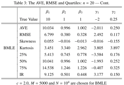
The results are given in Table 3, where BMLE is compared with M2SE and MLE.

The case of n=20, M =5000 and N =10⁴is examined in Table 3.

A discussion on choice of M and N is given in Appendix 6.1.6, where we examine

whether M =5000 and N = 10⁴are sufficient.

Table 3: The AVE, RMSE and Quartiles: n=20

β1 β2 β3 γ1 γ2

True Value 10 1 1 −2 0.25

AVE 10.064 0.995 1.002 −0.988 0.199 RMSE 7.537 0.418 0.333 3.059 0.146 Skewness 0.062 −0.013 −0.010 −0.101 −0.086 M2SE Kurtosis 4.005 3.941 2.988 3.519 3.572 25% 5.208 0.728 0.778 −2.807 0.113 50% 10.044 0.995 1.003 −0.934 0.200 75% 14.958 1.261 1.227 0.889 0.287

Table 3: The AVE, RMSE and Quartiles: n=20 — Cont.

β1 β2 β3 γ1 γ2

True Value 10 1 1 −2 0.25

AVE 10.029 0.997 1.002 −2.753 0.272 RMSE 7.044 0.386 0.332 2.999 0.139 Skewness 0.081 −0.023 −0.014 0.006 −0.160 MLE Kurtosis 4.062 3.621 2.965 4.620 4.801 25% 5.323 0.741 0.775 −4.514 0.189 50% 10.066 0.998 1.002 −2.710 0.273 75% 14.641 1.249 1.229 −0.958 0.355

IR 9.318 0.509 0.454 3.556 0.165

Table 3: The AVE, RMSE and Quartiles: n=20 — Cont.

β1 β2 β3 γ1 γ2

True Value 10 1 1 −2 0.25

AVE 10.034 0.996 1.002 −2.011 0.250 RMSE 6.799 0.380 0.328 2.492 0.117 Skewness 0.055 −0.016 −0.013 −0.016 −0.155 BMLE Kurtosis 3.451 3.340 2.962 3.805 3.897 25% 5.413 0.745 0.778 −3.584 0.176 50% 10.041 0.996 1.002 −1.993 0.252 75% 14.538 1.246 1.226 −0.407 0.325

IR 9.125 0.501 0.448 3.177 0.150

First, we compare the two traditional estimators, i.e., M2SE and MLE.

Judge, Hill, Griffiths and Lee (1980, pp.141–142) indicated that 2SE of γ1 is in- consistent although 2SE of the other parameters is consistent but asymptotically inefficient.

For M2SE, the estimate ofγ1 is modified to be consistent.

But M2SE is still asymptotically inefficient while MLE is consistent and asymptot- ically efficient.

Therefore, for γ, MLE should have better performance than M2SE in the sense of efficiency.

In Table 3, for all the parameters except for IR ofβ3, RMSE and IR of MLE are smaller than those of M2SE.

For both M2SE and MLE, AVEs ofβare close to the true parameter values.

Therefore, it might be concluded that M2SE and MLE are unbiased for βeven in the case of small sample.

However, the estimates of γ are different from the true values for both M2SE and MLE.

That is, AVE and 50% of γ1 are −0.988 and −0.934 for M2SE, and −2.753 and

−2.710 for MLE, which are far from the true value−2.0.

Similarly, AVE and 50% of γ2 are 0.199 and 0.200 for M2SE, which are different from the true value 0.25.

But 0.272 and 0.273 for MLE are slightly larger than 0.25 and they are close to 0.25.

Thus, the traditional estimators work well for the regression coefficientsβbut not for the heteroscedasticity parametersγ.

Next, the Bayesian estimator (i.e., BMLE) is compared with the traditional ones (i.e., M2SE and MLE).

For all the parameters of β, we can find from Table 3 that BMLE shows better

performance in RMSE and IR than the traditional estimators, because RMSE and IR of BMLE are smaller than those of M2SE and MLE.

Furthermore, from AVEs of BMLE, we can see that the heteroscedasticity parame- ters as well as the regression coefficients are unbiased in the small sample.

Thus, Table 3 also shows the evidence that for both β and γ, AVE and 50% of BMLE are very close to the true parameter values.

The values of RMSE and IR also indicate that the estimates are concentrated around the AVE and 50%, which are vary close to the true parameter values.

For the regression coefficientβ, all of the three estimators are very close to the true

parameter values. However, for the heteroscedasticity parameterγ, BMLE shows a good performance but M2SE and MLE are poor.

The larger values of RMSE for the traditional counterparts may be due to “outliers”

encountered with the Monte Carlo experiments.

This problem is also indicated in Zellner (1971, pp.281).

Compared with the traditional counterparts, the Bayesian approach is not charac- terized by extreme values for posterior modal values.

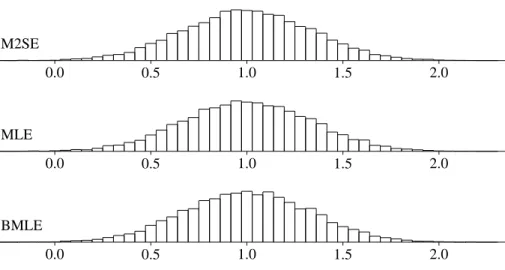
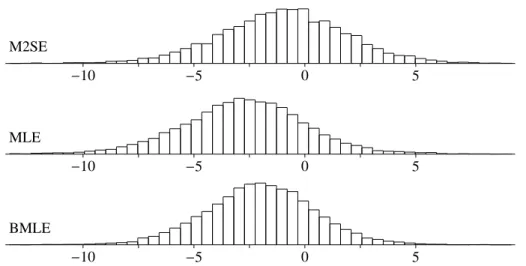
Now we compare empirical distributions for M2SE, MLE and BMLE in Figures 3 – 7.

Figure 3: Empirical Distributions ofβ1

M2SE

−15 −10 −5 0 5 10 15 20 25 30 35

MLE

−15 −10 −5 0 5 10 15 20 25 30 35

BMLE

Figure 4: Empirical Distributions ofβ2

M2SE

−0.5 0.0 0.5 1.0 1.5 2.0

MLE

−0.5 0.0 0.5 1.0 1.5 2.0

BMLE

Figure 5: Empirical Distributions ofβ3

M2SE

0.0 0.5 1.0 1.5 2.0

MLE

0.0 0.5 1.0 1.5 2.0

BMLE

Figure 6: Empirical Distributions ofγ1

M2SE

−10 −5 0 5

MLE

−10 −5 0 5

BMLE

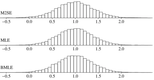
Figure 7: Empirical Distributions ofγ2

M2SE

−0.2 −0.1 0.0 0.1 0.2 0.3 0.4 0.5 0.6 0.7

MLE

−0.2 −0.1 0.0 0.1 0.2 0.3 0.4 0.5 0.6 0.7

BMLE

For the posterior densities of β1 (Figure 3), β2 (Figure 4), β3 (Figure 5) and γ1

(Figure 6), all of M2SE, MLE and BMLE are almost symmetric (also, see Skewness in Table 3).

For the posterior density ofγ2(Figure 7), both MLE and BMLE are slightly skewed to the left because Skewness of γ2 in Table 3 is negative, while M2SE is almost symmetric.

As for Kurtosis, all the empirical distributions except for β3 have a sharp kurtosis and fat tails, compared with the normal distribution.

Especially, for the heteroscedasticity parameters γ1 and γ2, MLE has the largest

kurtosis of the three.

For all figures, location of the empirical distributions indicates whether the estima- tors are unbiased or not.

Forβ1 in Figure 3, β2 in Figure 4 andβ3 in Figure 5, M2SE is biased while MLE and BMLE are distributed around the true value.

Forγ1 in Figure 6 andγ2 in Figure 7, the empirical distributions of M2SE, MLE and BMLE are quite different.

For γ1 in Figure 6, M2SE is located in the right-hand side of the true parameter value, MLE is in the left-hand side, and BMLE is also slightly in the left-hand side.

Moreover, for γ2 in Figure 7, M2SE is downward-biased, MLE is overestimated, and BMLE is distributed around the true parameter value.

On the Sample Size n: Finally, we examine how the sample size n influences precision of the parameter estimates.

Since we utilize the exogenous variable X shown in Judge, Hill, Griffiths and Lee (1980), we cannot examine the case where n is greater than 20.

In order to see the effect of the sample size n, here the case of n = 15 is compared with that of n= 20.

The case n = 15 of BMLE is shown in Table 4, which should be compared with BMLE in Table 3.

As a result, all the AVEs are very close to the corresponding true parameter values.

Therefore, we can conclude from Tables 3 and 4 that the Bayesian estimator is unbiased even in the small sample such as n=15,20.

However, RMSE and IR become large as n decreases.

That is, for example, RMSEs of β1, β2, β3, γ1 and γ2 are given by 6.799, 0.380, 0.328, 2.492 and 0.117 in Table 3, and 8.715, 0.455, 0.350, 4.449 and 0.228 in Table 4.

Thus, we can see that RMSE and IR decrease as n is large.

Table 4: BMLE: n=15, c=2.0, M=5000 and N =10⁴

β1 β2 β3 γ1 γ2

True Value 10 1 1 −2 0.25

AVE 10.060 0.995 1.002 −2.086 0.252 RMSE 8.715 0.455 0.350 4.449 0.228 Skewness 0.014 0.033 −0.064 −0.460 0.308 Kurtosis 3.960 3.667 3.140 4.714 4.604 25% 4.420 0.702 0.772 −4.725 0.107 50% 10.053 0.995 1.004 −1.832 0.245 75% 15.505 1.284 1.237 0.821 0.391

6.1.5 Summary

In Section 6.1, we have examined the multiplicative heteroscedasticity model dis- cussed by Harvey (1976), where the two traditional estimators are compared with the Bayesian estimator.

For the Bayesian approach, we have evaluated the posterior mean by generating random draws from the posterior density, where the Markov chain Monte Carlo methods (i.e., the MH within Gibbs algorithm) are utilized.

In the MH algorithm, the sampling density has to be specified.

We examine the multivariate normal sampling density, which is the independence

chain in the MH algorithm.

For mean and variance in the sampling density, we consider using the mean and variance estimated by the two traditional estimators (i.e., M2SE and MLE).

The Bayesian estimators with M2SE and MLE are called BM2SE and BMLE in Section 6.1.

Through the Monte Carlo studies, the results are summarized as follows:

(i) We compare BM2SE and BMLE with respect to the acceptance rates in the MH algorithm.

which is shown in Figure 2.

For the sampling density, we utilize the independence chain through Section 6.1.

The high acceptance rate implies that the chain travels over the support of the target density.

For the Bayesian estimator, therefore, BMLE is preferred to BM2SE.

However, note as follows.

The sampling density which yields the highest acceptance rate is not neces-

sarily the best choice and the tuning parameter c should be larger than the value which gives us the maximum acceptance rate.

Therefore, we have focused on BMLE with c = 2 (remember that BMLE with c= 1.2 yields the maximum acceptance rate).

(ii) For the traditional estimators (i.e., M2SE and MLE), we have obtained the result that MLE has smaller RMSE than M2SE for all the parameters, because for one reason the M2SE is asymptotically less efficient than the MLE.

Furthermore, for M2SE, the estimates of β are unbiased but those of γ are different from the true parameter values (see Table 3).

(iii) From Table 3, BMLE performs better than the two traditional estimators in the sense of RMSE and IR, because RMSE and IR of BMLE are smaller than those of the traditional ones for all the cases.

(iv) Each empirical distribution is displayed in Figures 3 – 7.

The posterior densities of almost all the estimates are distributed to be sym- metric (γ2is slightly skewed to the left), but the posterior densities of both the regression coefficients (except for β3) and the heteroscedasticity parameters have fat tails.

Also, see Table 3 for skewness and kurtosis.

(v) As for BMLE, the case of n =15 is compared with n= 20.

The case n= 20 has smaller RMSE and IR than n=15, while AVE and 50%

are close to the true parameter values forβandγ.

Therefore, it might be expected that the estimates of BMLE go to the true parameter values as n is large.

6.1.6 Appendix: Are M= 5000 and N =10⁴Sufficient?

Table 5: BMLE: n=20 and c=2.0

β1 β2 β3 γ1 γ2

True Value 10 1 1 −2 0.25

AVE 10.028 0.997 1.002 −2.008 0.250 RMSE 6.807 0.380 0.328 2.495 0.117 Skewness 0.041 −0.007 −0.012 0.017 −0.186 M=1000 Kurtosis 3.542 3.358 2.963 3.950 4.042 N =10⁴ 25% 5.413 0.745 0.778 −3.592 0.176 50% 10.027 0.996 1.002 −1.998 0.252 75% 14.539 1.245 1.226 −0.405 0.326

Table 5: BMLE: n=20 and c=2.0 — Cont.

β1 β2 β3 γ1 γ2

True Value 10 1 1 −2 0.25

AVE 10.033 0.996 1.002 −2.010 0.250 RMSE 6.799 0.380 0.328 2.491 0.117 Skewness 0.059 −0.016 −0.011 −0.024 −0.146 M=5000 Kurtosis 3.498 3.347 2.961 3.764 3.840 N =5000 25% 5.431 0.747 0.778 −3.586 0.176 50% 10.044 0.995 1.002 −1.997 0.252 75% 14.532 1.246 1.225 −0.406 0.326

In Section 6.1.4, only the case of (M,N)=(5000,10⁴) is examined.

In this appendix, we check whether M =5000 and N =10⁴are sufficient.

For the burn-in period M, there are some diagnostic tests, which are discussed in Geweke (1992) and Mengersen, Robert and Guihenneuc-Jouyaux (1999).

However, since their tests are applicable in the case of one sample path, we cannot utilize them.

Because G simulation runs are implemented in Section 6.1.4 (see p.516 for the simulation procedure), we have G test statistics if we apply the tests.

It is difficult to evaluate G testing results at the same time.

Therefore, we consider using the alternative approach to see if M = 5000 and N = 10⁴are sufficient.

For choice of M and N, we consider the following two issues.

(i) Given fixed M = 5000, compare N =5000 and N =10⁴. (ii) Given fixed N =10⁴, compare M =1000 and M= 5000.

(i) examines whether N = 5000 is sufficiently large, while (ii) checks whether M = 1000 is large enough. If the case of (M,N) =(5000,5000) is close to that of (M,N)=(5000,10⁴), we can conclude that N =5000 is sufficiently large.

Similarly, if the case of (M,N) = (1000,10⁴) is not too different from that of (M,N)=(5000,10⁴), it might be concluded that M =1000 is also sufficient.

The results are in Table 5, where AVE, RMSE, Skewness, Kurtosis, 25%, 50%, 75%

and IR are shown for each of the regression coefficients and the heteroscedasticity parameters.

BMLE in Table 3 should be compared with Table 5.

From Tables 3 and 5, the three cases, i.e., (M,N)=(5000,10⁴), (1000,10⁴), (5000,5000), are very close to each other.

Therefore, we can conclude that both M= 1000 and N = 5000 are large enough in

the simulation study shown in Section 6.1.4.

We take the case of M= 5000 and N= 10⁴for safety in Section 6.1.4, although we obtain the results that both M= 1000 and N =5000 are large enough.

6.2 Autocorrelation Model

In the previous section, we have considered estimating the regression model with the heteroscedastic error term, where the traditional estimators such as MLE and M2SE are compared with the Bayesian estimators.

In this section, using both the maximum likelihood estimator and the Bayes estima-

tor, we consider the regression model with the first order autocorrelated error term, where the initial distribution of the autocorrelated error is taken into account.

As for the autocorrelated error term, the stationary case is assumed, i.e., the auto- correlation coefficient is assumed to be less than one in absolute value.

The traditional estimator (i.e., MLE) is compared with the Bayesian estimator. Uti- lizing the Gibbs sampler, Chib (1993) discussed the regression model with the au- tocorrelated error term in a Bayesian framework, where the initial condition of the autoregressive process is not taken into account.

In this section, taking into account the initial density, we compare the maximum

likelihood estimator and the Bayesian estimator.

For the Bayes estimator, the Gibbs sampler and the Metropolis-Hastings algorithm are utilized to obtain random draws of the parameters.

As a result, the Bayes estimator is less biased and more efficient than the maxi- mum likelihood estimator. Especially, for the autocorrelation coefficient, the Bayes estimate is much less biased than the maximum likelihood estimate.

Accordingly, for the standard error of the estimated regression coefficient, the Bayes estimate is more plausible than the maximum likelihood estimate.

6.2.1 Introduction

In Section 6.2, we consider the regression model with the first order autocorrelated error term, where the error term is assumed to be stationary, i.e., the autocorrelation coefficient is assumed to be less than one in absolute value.

The traditional estimator, i.e., the maximum likelihood estimator (MLE), is com- pared with the Bayes estimator (BE).

Utilizing the Gibbs sampler, Chib (1993) and Chib and Greenberg (1994) discussed the regression model with the autocorrelated error term in a Bayesian framework, where the initial condition of the autoregressive process is ignored.

Here, taking into account the initial density, we compare MLE and BE, where the Gibbs sampler and the Metropolis-Hastings (MH) algorithm are utilized in BE.

As for MLE, it is well known that the autocorrelation coefficient is underestimated in small sample and therefore that variance of the estimated regression coefficient is also biased.

See, for example, Andrews (1993) and Tanizaki (2000, 2001).

Under this situation, inference on the regression coefficient is not appropriate, be- cause variance of the estimated regression coefficient depends on the estimated au- tocorrelation coefficient.

We show in Section 6.2 that BE is superior to MLE because BEs of both the auto- correlation coefficient and the variance of the error term are closer to the true values, compared with MLEs.

6.2.2 Setup of the Model

Let X_t be a 1×k vector of exogenous variables andβbe a k×1 parameter vector.

Consider the following regression model:

y_t =X_tβ+u_t, u_t =ρu_t−1+t, t ∼N(0, σ²),

for t = 1,2,· · ·,n, where 1, 2, · · ·, n are assumed to be mutually independently

distributed.

In this model, the parameter to be estimated is given byθ=(β,ρ,σ²).

The unconditional density of y_t is:

f (y_t|β, ρ, σ²)= 1

√2πσ²/(1−ρ²)exp(

− 1

2σ²/(1−ρ²)(y_t−X_tβ)²) . Let Y_t be the information set up to time t, i.e., Y_t = {y_t,y_t−1,· · ·,y₁}. The conditional density of y_t given Y_t−1is:

f (y_t|Y_t−1, β, ρ, σ²)= f (y_t|y_t−1, β, ρ, σ²)

= 1

√ exp(

− 1

σ ((y_t−ρy_t−1)−(X_t−ρX_t−1)β)²) .

Therefore, the joint density of Y_n, i.e., the likelihood function, is given by : f (Y_n|β, ρ, σ²)= f (y₁|β, ρ, σ²)

∏n t=2

f (y_t|Y_t−1, β, ρ, σ²)

= (2πσ²)^−n/2(1−ρ²)^1/2exp(

− 1 2σ²

∑n t=1

(y^∗_t −X_t^∗β)²)

, (20) where y^∗_t and X_t^∗represent the following transformed variables:

y^∗_t = y^∗_t(ρ)=



√1−ρ²y_t, for t= 1,

y_t−ρy_t−1, for t= 2,3,· · ·,n,

X_t^∗ =X_t^∗(ρ)=



√1−ρ²X_t, for t= 1,

X_t−ρX_t−1, for t= 2,3,· · ·,n, which depend on the autocorrelation coefficientρ.

Maximum Likelihood Estimator: We have shown above that the likelihood func- tion is given by equation (20).

Maximizing equation (20) with respect toβandσ², we obtain the following expres- sions:

βˆ ≡βˆ(ρ)= (

∑n

X_t^∗0X_t^∗)⁻¹

∑n

X_t^∗0y^∗_t,