Robust and Efficient Prediction with StructuralConstraints

Robust and Efficient Prediction with Structural Constraints

森富, 賢一郎

https://doi.org/10.15017/1931929

出版情報：九州大学, 2017, 博士（情報科学）, 課程博士 バージョン：

権利関係：

Constraints

Ken-ichiro Moridomi

February, 2018

Many real-world problems can be formulated as problems of predicting and learning objects with some structural constraints. In this thesis we handle two standard models of machine learning problem formulations. One is the online prediction model and the other is the statis- tical learning model. Online prediction is a theoretical model of repeated processes of making decisions, receiving feedbacks and incurring the loss defined by feedbacks and decisions. The goal of the algorithm is to perform nearly as well as the best decision in hindsight, where the best decision is determined by the feedback sequence. On the other hand, in the statistical learning model, the algorithm is given a set of labeled instances which are generated according to a probability distribution and then predicts a function called the hypothesis which maps an instance to a label. The goal of the algorithm is to minimize the probability that the hypothesis makes a wrong label.

We consider various formulations of machine learning problems with some structural con- straints. The motivation to introduce constraints is that many problems can be naturally and/or well formulated as optimization problems whose feasible solutions should satisfy some struc- tural constraints, where by structural constraints we mean combinatorial constraints or algebraic constraints.

For example, a network routing problem is naturally formulated as an online prediction problem where decisions made by the algorithm are restricted to paths or spanning trees of a graph. Another example is a recommendation by ranking, where the decisions are restricted to permutations over the set of items under consideration.

As for the algebraic constraints, we consider the matrix completion problem under the both

models of online prediction and statistical learning. The most common application of the matrix

completion is the collaborative filtering, which can be viewed as the problem of matrix comple-

tion of the preference matrix. One of the most successful method is to put a low rank or a low

matrix norm constraint on the space of matrices for the algorithm to choose from [70, 72].

we require algorithms to perform well against the worst-case environment. For the efficiency, we require algorithms to run in polynomial time.

There are four main results in this thesis. First, we consider an online prediction task of matrices. The reduction technique from some online prediction tasks of matrices to online pre- diction of symmetric positive semi-definite matrices (shortly online SDP problems) [38], and a framework of designing an algorithm [36]were known. The algorithm based framework of [36] makes prediction as minimize the cumulative loss and a convex function called the regu- larizer simultaneously. We develop a new technique of analyzing algorithms with introducing new notion of the strong convexity of the regularizer. We suggest an algorithm using the log- determinant as the regularizer for a online SDP problem, and analyze it with our new technique.

We improve the performance measure of the algorithm and is optimal in some online prediction tasks. Next, we handle the binary matrix completion problem in online and statistical learning model. We introduce the new notion for measuring the difficulty of the data which the algorithm receives, and reduce the online binary matrix completion problem to the online SDP problem.

And then apply our algorithm proposed in previous chapter. We improve the upper bound of mistakes that the algorithm will make and has the optimal mistake bound We can apply this algorithm to the statistical learning setting. In the statistical learning setting, our algorithm competes with the Support Vector Machine with the best feature mapping without knowing the feature map. Thirdly, we propose new classes of matrices for the matrix completion prob- lem. The new class of matrices defined by matrix factorization with norm constraints. We give generalization error bounds for these matrix classes. We also show some experimental results.

Finally, we develop an algorithm for the Metrical Task System problem (shortly MTS problem)

of combinatorial objects. In combinatorial setting, the number of the decision grows exponen-

tially of some domain and the na¨ıve implementation of the algorithms for the MTS problem

leads exponential time algorithms. We reduce the bottleneck of Marking algorithm [16] to a

sampling problem over combinatorial objects. Combining sampling oracles, our algorithm is

the first efficient time algorithm for this problem under the uniform metric. We derive its per-

formance measure and give a proof of the optimality of our algorithm in some specific case of

the combinatorial objects.

I would like to show my gratitude for everyone’s support while studying. First of all I am extremely grateful for Professor Eiji Takimoto. He is my supervisor and the committee chair of this thesis. His deep understanding and strictly theoretical thinking of mathematics, machine learning and computational theory made me grow up a lot. His ideas based on theoretical point of view always helps me and became breakthroughs of my research. I also would like to thank Professor Jun’ichi Takeuchi and Associate Professor Shuji Kijima, who gave me many valuable comments as committee members of this thesis.

I greatly appreciate to Professor Kohei Hatano. He gave me many valuable advice not only for my research but also for my career as a researcher. He also supported me in the programming field. I also appreciate to Professor Masayuki Takeda, Professor Hideo Bannai and Professor Shunsuke Inenaga for their advice in weekly seminars. Their advice greatly improve my presentation skill. Professor Takeda also gave me many valuable advice for my job hunting.

The results in this thesis were published in proceedings of ACML 2014 [59], proceedings of ALT 2016 [60]. The journal version of ACML 2014 with some refinement of analysis will be published in The IEICE Transactions on Information and Systems. Its arXiv e-print is available in [58]. I appreciate all editors, committees, anonymous referees, and publishers.

I am also grateful to the technical staffs of our laboratory, Ms. Sanae Wakita, Ms. Miho Higo, Ms. Akiko Ikeuchi and Ms. Yuko Hasegawa. They always supported me in many situ- ations not only paperwork. I also express thanks to all of staffs in Department of Informatics, Kyushu University.

Last, but not least, I really thank my family for their support.

Abstract i

Acknowledgements iii

1 Introduction 1

1.1 Our contributions . . . . 2

1.2 Organization . . . . 6

2 Preliminaries 7 2.1 Notations . . . . 7

2.2 Statistical learning model . . . . 8

2.3 Online learning model . . . . 9

2.4 Well-known formulas . . . . 11

3 Online linear optimization with the log-determinant regularizer 12 3.1 Introduction . . . . 12

3.2 Problem setting . . . . 15

3.3 FTRL and its regret bounds by standard derivations . . . . 16

3.4 Online matrix prediction and reduction to online SDP . . . . 23

3.5 Main results . . . . 26

3.6 Conclusion . . . . 36

4 Optimal mistake bounds for binary matrix completion the log-determinant regu- larization 37 4.1 Introduction . . . . 37

4.2 Related work . . . . 38

4.3 Preliminaries . . . . 39

4.4 Reduction of the binary matrix prediction . . . . 40

4.5 Our algorithm and analysis . . . . 44

4.6 Connection to the batch setting . . . . 47

4.7 Implementation details . . . . 50

4.8 Conclusion . . . . 52

5 Tighter generalization error bounds for matrix completion 53 5.1 Introduction . . . . 53

5.2 Related work . . . . 55

5.3 Problem setting . . . . 56

5.4 Generalization bounds for our hypothesis classes . . . . 60

5.5 A matching lower bound on the Rademacher complexity . . . . 64

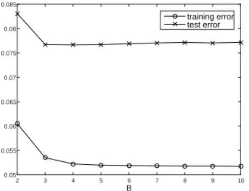
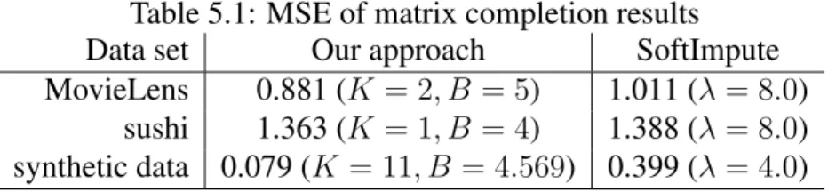
5.6 Experimental results . . . . 67

5.7 Conclusion . . . . 69

5.8 Implementation details . . . . 70

5.9 Yet another proof of Lemma 16 . . . . 70

6 A Combinatorial Metrical Task System Problem under the Uniform Metric 72 6.1 Introduction . . . . 72

6.2 Preliminaries . . . . 74

6.3 The Marking algorithm . . . . 75

6.4 The Weighted Marking algorithm . . . . 77

6.5 Conclusion and future work . . . . 85

7 Conclusion 86

Introduction

Machine learning is used in many fields, and there are various problem formulations of machine learning problems. In particular, many real-world problems can be formulated as the problems of predicting and learning objects with some structural constraints. In this thesis we handle two standard models of machine learning problem formulations. One is the online prediction model and the other is the statistical learning model.

Online prediction is a theoretical model of repeated processes of making decisions, receiving feedbacks and incurring the loss defined by feedbacks and decisions. Each repeat is called the round. This type of problem has been extensively studied in the machine learning community for a couple of decades [27, 44, 23]. The goal of the algorithm is to perform nearly as well as the best decision in hindsight, where the best decision is determined by the feedback sequence.

In particular, we consider two measures to evaluate the algorithm performance relative to the best decision. One is the regret which is defined as the difference of the cumulative loss of the algorithm and that of the best decision, and the other is the competitive ratio which is defined as the ratio of them.

On the other hand, in the statistical learning model, the algorithm is given a set of labeled instances (where the label of each instance represents its correct classification) which are gen- erated according to a probability distribution and then predicts a function called the hypothesis which maps an instance to a label. The goal of the algorithm is to minimize the generaliza- tion error, the probability that the hypothesis makes a wrong label. This model is called the Probably Approximately Correct learning (PAC learning, for short) framework [75]. One of the major issues of the PAC learning framework is to give theories for analyzing the generalization error and has been extensively studied until now [78, 5].

We consider various formulations of machine learning problems with some structural con-

straints. The motivation to introduce constraints is that many problems can be naturally and/or well formulated as optimization problems whose feasible solutions should satisfy some struc- tural constraints, where by structural constraints we mean combinatorial constraints or algebraic constraints.

For example, a network routing problem is naturally formulated as an online prediction problem where decisions made by the algorithm are restricted to paths or spanning trees of a graph. Another example is a recommendation by ranking, where the decisions are restricted to permutations over the set of items under consideration. In these cases, the algorithm is required to choose a combinatorial object as the prediction.

As for the algebraic constraints, we consider a particular problem, the matrix completion, under the both models of online prediction and statistical learning. Intuitively, the matrix com- pletion problem is to predict the whole entries of a matrix from partial entries given. The most common application of the matrix completion is the collaborative filtering, where the task is to predict the preferences of m users over n items from partial information, which can be viewed as the problem of matrix completion of the m × n preference matrix. One of the most successful method is to put a low rank or a low matrix norm constraint on the space of matrices for the algorithm to choose from [70, 72].

Our aim in this thesis is to develop the methods of designing and analyzing algorithms for predicting objects with some structural constraints, so that they are robust and efficient. For the robustness, we require algorithms to perform well against the worst-case environment. For the efficiency, we require algorithms to run in polynomial time.

1.1 Our contributions

In this section, we briefly describe the problems we consider in this thesis and show related work and our contribution.

1.1.1 Online semi-definite programming problem

Modeling with matrices is more natural than modeling with vectors for some applications such

as ranking and recommendation tasks [20, 39, 42]. Hazan et.al. [38] show that some online

prediction problem of matrices related to ranking and recommendation can be reduced to an

online prediction problem of symmetric positive semi-definite matrices under linear loss func-

tions. Thus, we can focus on the online prediction problems for symmetric positive semi- definite matrices, which we call the online semi-definite programming (online SDP) problems.

In the online SDP problem, the algorithm repeats the following round: first chooses a symmet- ric positive semi-definite matrix from an bounded set, then receives a symmetric matrix from an environment and finally incurs the loss defined as the inner product of chosen matrix and received matrix. The goal of the algorithm is to minimize the regret, the difference between the cumulative loss of the algorithm and that of the best fixed matrix in hindsight in the bounded set.

On the online prediction tasks, there is a standard framework called Follow the Regularized Leader (FTRL) for designing and analyzing algorithms [36, 65, 68, 37], where we need to choose as a parameter an appropriate function called regularizer.

Hazan et.al.˜propose an algorithm for the online SDP problems which employ the von Neu- mann entropy as the regularizer, and shows that the O( √

T βτ ln N ) of the upper bound of the regret where β, τ are bounding parameter of the algorithm’s predictions, N is the size of the ma- trices and T is the number of rounds. However, their algorithm turns out to be sub-optimal [38].

Another possible choice of the regularizer is the log-determinant. Christiano uses the log- determinant as the regularizer and considers a very specific sub-class of online SDP problems and succeeds to improve the regret bound for a particular application problem [21]. But the problems he examines do not cover the whole class of online prediction tasks which admit the reduction to online SDP problems.

In this thesis, we propose an algorithm for the online SDP problems which uses the log- determinant regularization. We extend the analysis of Christiano in [21] and develop a new technique of deriving regret bounds by exploiting the new notion of the strong convexity of the regularizer. The analysis in [21] is not explicitly stated as in a general form and focused on a very specific case. We improve the regret bound for online SDP problem when feedback matrices are sparse, and show the O( √

T βτ ) of the upper bound of the regret which is optimal for some application problems proposed in [38].

1.1.2 Online binary matrix completion problem

Learning preferences of users over a set of items is an important task in recommendation sys-

tems. In particular, the collaborative filtering approach is known to be quite effective and pop-

ular [66, 52, 80]. The approach is formulated as the matrix completion problem, where, an

underlying matrix represents user’s preferences of items, only some entries of the matrix are given and the goal is to predict rest of preferences. Under the natural assumption that captures the low rank property of the matrix, a lot of work have been done in various settings, say, the statistical i.i.d. setting [71, 31, 69, 56] and the online learning setting [20, 38, 59, 42]

The online binary matrix completion problem posed by Herbseter et al. [39] is defined in the following way. The problem is defined as a series of round. For each round, the algorithm receives a pair of a user and an item, then predicts that the user likes given item or not and finally incurs the loss if the prediction is wrong. The goal of the algorithm is to minimize the total loss (i.e. the number of errors).

Herbster et al. [39] considered an online version of the binary matrix completion problem and give an algorithm. Their analysis introduce the margin complexity of the matrix, an differ- ent aspects of the complexity of the matrix from the matrix rank. Their algorithm enjoys the mistake bounds of O(

γ²

) for the problem, where the m,n are the numbers of users and items respectively and γ is the margin complexity. However, their mistake bound is not optimal yet.

For the online binary matrix completion problem, we propose an FTRL-based algorithm with the log-determinant regularizer and prove mistake bounds of the algorithm under a natural assumption of [39]. We develop a sharper reduction technique from the online binary matrix completion to the online SDP problem [38] and apply of a modified notion of the strong con- vexity mentioned in previous subsection for the log-determinant [59, 58].

The mistake bounds of our algorithm O(

) are optimal,

We also apply our online algorithm in the statistical learning model by a standard online to batch conversion framework (see, e.g., [57]), and derive a generalization error bound. In this setting, we also can drop the logarithmic factor from the result of [39]. Our generalization error bound is similar to the known margin-based bound obtained by the best kernel in hindsight.

Additionally, we introduce the standard notion of the margin loss [57] to measure the difficulty of the given sample in the both settings. This is a tighter measure than the margin error.

1.1.3 Matrix factorization under norm constraints

We studied the matrix completion problem in statistical machine learning setting, that is, learn-

ing a user-item rating matrix from given sample. The sample consists partial entries of the

matrix. Different from previous result, in this problem, the algorithm requires to predict user’s

ratings in the real value (not binary). A common assumption in the previous work is that the true matrix X ∈ R

can be well approximated by a matrix of low rank matrix X = UV ˆ

(or low trace norm, as a convex relaxation of the rank constraint). Generalization ability of algorithms (such as the empirical risk minimization) using low rank or low trace norm matrices is intensively studied in the literature (see, e.g., [70, 71, 72, 31]).

Recently, further additional constraints on the class of hypothesis matrices turns out to be effective in practice. In particular, a major approach is to impose the constraints that U and V are non-negative with bounded L

norm [51, 48, 33, 79, 54, 28]. Such a decomposition is called the non-negative matrix factorization (NMF, for short). A typical scheme of the NMF approach is the empirical risk minimization with the norm regularization [48, 33, 28]. Despite the empirical success of the NMF approach, no theoretical justification has been given.

In this thesis, we consider different but closely related classes of hypothesis matrices and give generalization bounds of these classes. Our bounds are of O( √

(nK + m log K )/T ), where T is the sample size and K is the rank of X. These bounds improve the previously ˆ known bound O( ˜ √

(n + m)K/T ) that is derived for the class where only the low-rank con- straint is imposed [70]. Therefore, our results would give theoretical evidence for the empirical success of the NMF. However, our new bounds hold even when U and V have negative values in some components. This result suggests that our analysis may not yet fully capture the prop- erty of the non-negativity constraint, or the empirical success of the NMF may not rely on the non-negativity very much but mostly on the regularization.

Our technical contributions are twofold. The first one is that we develop a new technique for bounding the Rademacher complexity to derive generalization bounds. The second one is that we prove a matching lower bound of the Rademacher complexity of the first hypothesis class. This means that our generalization bounds are tightest among those derived from the Rademacher complexity argument. There are few results in the literature on deriving lower bounds of the Rademacher complexity.

1.1.4 Combinatorial metrical task system problems

The metrical task system (MTS) problem is a scheme of the online learning model, it repeats the round (making decision and receive feedbacks) but it impose cost for changing the algorithm’s decision. The MTS problem is defined as a repeated game between the player and the adversary.

Consider a fixed set of states, a metric over the state set and a initial state. For each round,

the adversary reveals a (processing) cost function, then the algorithm chooses a state from the state set and finally the algorithm incurs the loss defined as the sum of the processing cost and the distance from previous state to current state. The goal of the algorithm is minimizing the cumulative (processing and moving) cost. The performance of the algorithm is measured by the competitive ratio, that is, the ratio of the cumulative cost of the algorithm to the cumulative cost of the best fixed sequence of states in hindsight. In the setting that the state set consists of n states, there are many existing works on the MTS [16, 40, 8, 29, 9] problem. In particular, for the uniform metric (which is defined as 1 if states are different and otherwise 0), the MTS problem is well studied [16, 8, 40, 1].

When we consider the situation where the state set is a combinatorial set from { 0, 1 }

, the computational issue arises. In general, for typical combinatorial sets, the size could be exponential in the dimension size d as well and straightforward implementations of known algorithms for the MTS problem take exponential time as well since time complexity of these algorithms is proportional to the size n = O(2

).

In this thesis, for the combinatorial MTS problem under the uniform metric, we propose a modification of the Marking algorithm [16], which employs an exponential weighting scheme.

We prove that our algorithm retains O(log n) competitive ratio for the standard MTS problem with n states. Combining with efficient sampling techniques w.r.t. exponential weights on combinatorial objects [73, 19, 41, 2], our algorithm works efficiently for various classes of combinatorial sets. We also give a lower bound of the competitive ratio in the case of that the state set is k-set. This result shows that our algorithm is optimal in this case.

1.2 Organization

The rest of this thesis is organized as follows: In Chapter 3 we consider an online prediction

problem of symmetric positive semi-definite matrices and propose a novel method for analyzing

online algorithms by introducing a new notion of strong convexity. In Chapter 4, we apply the

log-determinant regularization technique in the binary matrix completion problem, and show

the mistake bound. We also apply our online algorithm to the statistical learning setting and

derive a generalization error bound. In Chapter 5, we consider the matrix completion problem

and give a generalization error bound of the class defined by the matrix factorization with norm

constraints. In Chapter 6, we propose the first efficient algorithm for metrical task system

problems over combinatorial objects under the uniform metric.

Preliminaries

In this chapter, we define some notations to be used throughout this thesis and introduce three learning models, the statistical learning model, the online learning model.

2.1 Notations

In this thesis, matrices are denoted by roman capital letters. Let R

, S

, S

be the set of m × n matrices, the set of N × N symmetric matrices, and the set of N × N symmetric positive semi-definite matrices, respectively.

For a matrix X, let σ

be its i-th largest singular value. We write the trace of a matrix X as Tr(X) and the determinant as det(X). We write its trace norm as ∥ X ∥

= ∑

i

σ

, spectral norm as ∥ X ∥

= max

σ

, and Frobenius norm as ∥ X ∥

= √∑

i

σ

. For the matrix X, we write its largest eigenvalue and smallest eigenvalue by λ

(X) and λ

(X), respectively.

We write the identity matrix as E. The notion X ⪰ 0 means X is positive semi-definite. For any positive integer m, we write [m] = { 1, 2, . . . , m } . We define the vectorization of a matrix X ∈ R

as

vec(X) = (X

, X

, . . . , X

)

,

where X

is the i-th column of X. For m × n matrices X and L, X • L = ∑

∑

j=1

X

L

= vec(X)

vec(L) is the Frobenius inner product.

For a vector x ∈ R

, diag(x) denote the N × N diagonal matrix X such that X

= x

. For m × n matrices X and L, X • L = ∑

i,j

X

L

= vec(X)

vec(L) is the Frobenius inner product. For a matrix X, we write its i-th row as X

and j-th column as X

.

For a differentiable function R : R

→ R , its gradient ∇ R(X) is the m × n matrix whose

(i, j)-th component is

i,j

, and its Hessian [55, 30] ∇

R(X) is the mn × mn matrix defined by

( ∇

R(X))

= ∂

R(X)

∂X

∂X

.

We denote the Kronecker product of two matrices A ∈ R

and B ∈ R

as A ⊗ B ∈ R

, which is defined as (A ⊗ B)

= A

B

. We use the notation A ⊠ B ∈ R

as the box product of A and B, which is introduced by [30] and defined as (A ⊗ B)

= A

B

. These products have following properties [30]:

(A ⊗ B)vec(X) = vec(BXA

), (2.1)

(A ⊠ B)vec(X) = vec(BX

A

). (2.2) For a differentiable convex function R, the Bregman divergence with respect to R is defined as

B

(X, Y) = R(X) − R(Y) − ∇ R(Y) • (X − Y).

2.2 Statistical learning model

The statistical learning model is one of the most important model in machine learning. In this model, the algorithm given a set of randomly generated data called the sample set, and then required to produce a function called as the hypothesis which maps a data to the label. The performance of the algorithm is measured by the generalization error of the hypothesis that the algorithm produced. Intuitively, the generalization error measures how well the hypothesis predicts labels for unseen data generated according to same distribution which generates the sample set.

2.2.1 Problem setting

Let X and Y be the input space and the label space, respectively. Let a sequence S = ((x

, y

), (x

, y

), . . . , (x

, y

))

be a sample set where each (x

, y

) ∈ X × Y for t ∈ [T ] are generated independently according

to some unknown distribution D over X × Y . We call T as the size of S . The algorithm is

given a sample S and then required to produce a function h ∈ H maps X to Y . We call h

the hypothesis and H the hypothesis set. The goal of the algorithm is to produce h ∈ H that minimizes the generalization error as small as possible.

Let ℓ : Y × Y be a loss function, then the generalization error is defined as follows:

Definition 1 (Generalization error). For a hypothesis h : X → Y and distribution D The generalization error of h is

L(h) = E

[ℓ(h(x), y)].

If ℓ(x, y) = 1

then L(h) = Pr

[h(x) ̸ = y]. We cannot compute the generalization error due to unknown distribution D , but one can estimate it by the empirical error:

Definition 2 (Empirical error). For a hypothesis h : X → Y and a sample S of size T , the empirical error of h is

L(h) = ˆ 1 T

∑

ℓ(h(x), y).

Thus E

[ ˆ L(h)] = L(h).

2.3 Online learning model

The online learning model consists a series of repeated games between the algorithm and an (adversarial) environment. We study two types under this model, the online convex optimization and the metrical task system.

2.3.1 Online convex optimization

Online convex optimization is a repeated game between an algorithm and an adversarial envi- ronment.

Problem setting

In the online convex optimization, the following protocol proceeds; For each round t = 1, . . . , T , the algorithm (i) predicts x

∈ K , (ii) receives a convex function ℓ

: K → R and (iii) suffers the loss ℓ

(x

). The goal of the algorithm is to minimize the cumulative loss ∑

t=1

ℓ

(x

). In this thesis, in some cases, the loss function is the linear function ℓ

(x

) = ℓ

· x

. We regard the algorithm receives ℓ

instead of ℓ

and this problem was called the online linear optimization.

The regret is most standard measure of the performance of the algorithm.

Definition 3. Let x

, x

, . . . , x

∈ K be the predictions of the algorithm. The regret of the algorithm is

Reg(T, K , L , x

) =

∑

ℓ

(x

) −

∑

ℓ

(x

), where x

∈ K is a competitor.

Usually, the best offline solution x

= arg min

∑

t=1

ℓ

(x) was used as the competitor.

2.3.2 Metrical task system

The metrical task system takes into account a cost of changing decisions.

Problem setting

The metrical task system is defined by a set C and a metric function δ : C × C → R . In the metrical task system, first the adversary chooses a task sequence σ = (ℓ

, ℓ

, . . . , ℓ

), where each ℓ

: C → R is called a loss function. For a given initial state c

∈ C , in each round t = 1, . . . , T , the algorithm (i) receives ℓ

: K → R and (ii) chooses c

∈ C , (iii) suffers the cost ℓ

(x

) + δ(c

, c

). The first term ℓ

(c

) of the cost is called the processing cost at round t, and the second term δ(c

, c

) is called the moving cost at round t.

For a task sequence σ, the cumulative cost of an algorithm A is defined as cost

(σ) =

∑

(ℓ

(c

) + δ(c

, c

)),

and the cumulative cost of the best offline solution is defined as cost

(σ) = min

(c^∗₁,c^∗₂,...,c^∗_T)∈C^T

∑

(ℓ

(c

) + δ(c

, c

)).

We measure the performance of algorithm A by its competitive ratio, which is defined as CR(σ) = E [cost

(σ)]

cost

(σ) ,

where the expectation is with respect to the internal randomness of A. The goal of the algorithm

is to minimize the worst case competitive ratio max

CR(σ).

2.4 Well-known formulas

In this section we show well-known mathematical theorems we use in this thesis.

Definition 4 (Martingale difference). A sequence of random variables V

, V

, . . . is a martingale difference sequence with respect to X

, X

, . . . if for all t > 0, V

is a function of X

, . . . , X

and E [V

| X

, . . . , X

] = 0.

Theorem 1 (Azuma’s inequality). Let V

, V

, . . . be a martingale difference sequence with re- spect to the random variables X

, X

, . . .. Assume that for all t > 0, there is a constant c

and random variable Z

which is a function of X

, . . . , X

such that Z

≤ V

≤ Z

+ c

. Then, for all ϵ > 0 and T , following inequalities hold:

Pr[

∑

V

≥ ϵ] ≤ e

,

Pr[

∑

V

≤ − ϵ] ≤ e

.

Theorem 2 (McDirmid’s inequality). Let X

, . . . , X

∈ X

be a set of T ≥ 1 independent random variables and assume that ∃ c

, . . . , c

> 0 such that f : X

→ R satisfies

| f(x

, . . . , x

, . . . , x

) − f(x

, . . . , x

, . . . , x

) | ≤ c

for all t ∈ [T ] and any points x

, . . . , x

, x

.

Then the following inequality holds:

Pr[f (X

, . . . , X

) − E [f(X

, . . . , X

)] ≥ ϵ] ≤ e

,

Pr[f (X

, . . . , X

) − E [f(X

, . . . , X

)] ≤ − ϵ] ≤ e

.

Online linear optimization with the log-determinant regularizer

3.1 Introduction

Online prediction is a theoretical model of repeated processes of making decisions and receiving feedbacks, and has been extensively studied in the machine learning community for a couple of decades [27, 44, 23]. Typically, decisions are formulated as vectors in a fixed set called the decision space and feedbacks as functions that define the losses for all decision vectors.

Recently, much attention has been paid to a more general setting where decisions are formulated as matrices, since it is more natural for some applications such as ranking and recommendation tasks [20, 39, 42].

Take the online collaborative filtering as an example. The problem is formulated as in the following protocol: Assume we have a fixed set of n users and a fixed set of m items.

For each round t = 1, 2, . . . , T , the following happens. (i) The algorithm receives from the

environment a user-item pair (i

, j

), (ii) the algorithm predicts how much user i

likes item j

and chooses a number x

that represents the degree of preference, (iii) the environment returns

the true evaluation value y

of the user i

for the item j

, and then (iv) the algorithm suffers

loss defined by the prediction value x

and the true value y

, say, (x

− y

)

. Note that, (iii)

and (iv) in the protocol above can be generalized in the following way: (iii) the environment

returns a loss function ℓ

, say ℓ

(x) = (x − y

)

, and (iv) the algorithm suffers loss ℓ

(x

). The

goal of the algorithm is to minimize the cumulative loss, or more formally, to minimize the

regret, which is the most standard measure in online prediction. The regret is the difference

between the cumulative loss of the algorithm and that of the best fixed prediction policy in

some policy class. Note that the best policy is determined in hindsight, i.e., it depends on the whole feedback sequence. Now we claim that the problem above can be regarded as a matrix prediction problem: the algorithm chooses (before observing the pair (i

, j

)) the prediction values for all pairs as an m × n matrix, although only the (i

, j

)-th entry is used as the prediction.

In this perspective, the policy class is formulated as a restricted set of matrices, say, the set of matrices of bounded trace norm, which is commonly used in collaborative filtering [71, 56, 69, 47]. Moreover, we can assume without loss of generality that the prediction matrices are also chosen from the policy class. So, the policy class is often called the decision space.

In most application problems including the online collaborative filtering, the matrices to be predicted are not square, which makes the analysis difficult. Hazan et al. [38] show that any on- line matrix prediction problem formulated as in the protocol above can be reduced to an online prediction problem where the decision space consists of symmetric positive semi-definite ma- trices under linear loss functions. A notable property of the reduction is that the loss functions of the reduced problem are the inner product with sparse loss matrices, where only at most 4 entries are non-zero. Thus, we can focus on the online prediction problems for symmetric pos- itive semi-definite matrices, which we call the online semi-definite programming (online SDP) problems. In particular we are interested in the case where the problems are obtained by the reduction, which we call the online sparse SDP problems. Thanks to the symmetry and positive semi-definiteness of the decision matrices and the sparseness of the loss matrices, the problem becomes feasible and Hazan et al. propose an algorithm for the online sparse SDP problems, by which they give regret bounds for various application problems including the online max-cut, online gambling, and the online collaborative filtering [38]. Unfortunately, however, all these bounds turn out to be sub-optimal.

In this chapter, we propose an algorithm for the online sparse SDP problems by which we achieve optimal regret bounds for those application problems.

To this end, we employ a standard framework called Follow the Regularized Leader (FTRL)

for designing and analyzing algorithms [36, 65, 68, 37], where we need to choose as a parameter

an appropriate regularization function (or regularizer) to obtain a good regret bound. Hazan et

al. use the von Neumann entropy (or sometimes called the matrix negative entropy) as the

regularizer to obtain the results mentioned above [38], which is a generalization of Tsuda et

al. [74]. Another possible choice is the log-determinant regularizer, whose Bregman divergence

is so called the LogDet divergence. There are many applications of the LogDet divergence such

as metric learning [26], learning of low-rank kernels [50], clustering of multivariate Gaussians

[25], and Gaussian graphical models [67]. However, the log-determinant regularizer is less popular in online prediction and it is unclear how to derive general and non-trivial regret bounds when using the FTRL with the log-determinant regularizer, as posed as an open problem in [74].

Indeed, Davis et al. apply the FTRL with the log-determinant regularizer for square loss and give a cumulative loss bound [26], but it contains a data-dependent parameter and the regret bound is still unclear. Christiano considers a very specific sub-class of online sparse SDP problems and succeeds to improve the regret bound for a particular application problem, the online max-cut problem [21]. But the problems he examines do not cover the whole class of online sparse SDP problems and hence his algorithm cannot be applied to the online collaborative filtering, for instance.

We improve regret bounds for online sparse SDP problems by analyzing the FTRL with the log-determinant regularizer. In particular, our contributions are summarized as follows.

1. We give a non-trivial regret bound of the FTRL with the log-determinant regularizer for a general class of online SDP problems. Although the bound seems to be somewhat loose, it gives a tight bound when the matrices are diagonal (which corresponds to the vector predictions).

2. We extend the analysis of Christiano in [21] and develop a new technique of deriving re- gret bounds by exploiting the property of strong convexity of the regularizer with respect to the loss matrices. The analysis in [21] is not explicitly stated as in a general form and focused on a very specific case where the loss matrices are block-wise sparse.

3. We improve the regret bound for the online sparse SDP problems, by which we give optimal regret bounds for the application problems, namely, the online max-cut, online gambling, and the online collaborative filtering.

4. We apply the results to the case where the decision space consists of vectors, which can

be reduced to online matrix prediction problems where the decision space consists of

diagonal matrices. In this case, the general regret bound mentioned in 1 also gives tight

regret bound.

3.2 Problem setting

We first describe the problem setting: the online semi-definite programming problem (online SDP problem, for short).

3.2.1 Online SDP problem

We consider an online linear optimization problem over symmetric semi-definite matrices, which we call the online SDP problem. The problem is specified by a pair ( K , L ), where K ⊆ S

is a convex set of symmetric positive semi-definite matrices and L ⊆ S

is a set of symmetric matrices. The set K is called the decision space and L the loss space. The online SDP problem ( K , L ) is a repeated game between the algorithm and the adversary (i.e., an environment that may behave adversarially), which is described as the following protocol.

In each round t = 1, 2, . . . , T , the algorithm 1. chooses a matrix X

∈ K ,

2. receives a loss matrix L

∈ L from the adversary, and 3. suffers the loss X

• L

.

The goal of the algorithm is to minimize the regret Reg

(T, K , L , X

), defined as Reg

(T, K , L , X

) =

∑

L

• X

−

∑

L

• X

.

where X

∈ K is some competitor matrix.

If the competitor is the best matrix in the decision set K that minimizes the cumulative loss i.e. X

= arg min

∑

t=1

L

• X, the matrix X

is called the best offline matrix. In this case we abbreviate the argument X

and write Reg

(T, K , L ) = Reg

(T, K , L , X

).

3.2.2 Online linear optimization over vectors

The online SDP problem is a generalization of the online linear optimization problem over vectors, which is a more standard problem setting in the literature. For the “vector” case, the problem is described as the following protocol:

In each round t = 1, · · · , T , the algorithm

1. chooses x

∈ K ⊂ R

,

2. receives ℓ

∈ L ⊂ R

from the adversary, and 3. suffers the loss x

ℓ

.

It is easy to see that the problem is equivalent to the online SDP problem ( K

L

) where K

= { diag(x) | x ∈ K} and L

= { diag(ℓ) | ℓ ∈ L} . So, all the results for the online SDP problem can be applied to the online linear optimization over vectors.

3.3 FTRL and its regret bounds by standard derivations

Follow the Regularized Leader (FTRL) is a standard framework for designing algorithms for a wide class of online optimizations (see, e.g., [68]). To employ the FTRL, we need to specify a convex function R : K → R called the regularization function, or simply the regularizer.

For the online SDP problem ( K , L ), the FTRL with regularizer R suggests to choose a matrix X

∈ K as the decision at each round t according to

X

= arg min

X∈K

(

R(X) + η

∑

L

• X )

, (3.1)

where η > 0 is a constant called the learning rate. Note that we adopt X

= arg min

R(X), naturally induced by this rule. Throughout the thesis, we assume for simplicity that all the regularizers R are differentiable.

The FTRL has two closely related or equivalent formulation, which has the different form of from (3.1), and called as the Online Mirror Descent (OMD for short). Which is

X ˜

= ( ∇ R)

( ∇ R( ˜ X

) − ηL

) and X

= arg min

X∈K

B

(X, X ˜

), (3.2) X ˜

= ( ∇ R)

( ∇ R(X

) − ηL

) and X

= arg min

X∈K

B

(X, X ˜

), (3.3) where B

is the Bregman divergence with respect to R. The algorithm defined by (3.3) is called the lazy version and (3.3) is called the agile version [37]. We can say that if the loss function is linear then the lazy version of OMD is equivalent to the FTRL in (3.1).

Proposition 3 ([37]). Let B

be the Bregman divergence with respect to the convex function R.

For any online SDP problem ( K , L ), Let X ˜

= ( ∇ R)

( ∇ R( ˜ X

) − ηL

) where ( ∇ R)

is the

inverse function of ∇ R. Then

arg min

X∈K

R(X) + η

∑

L

• X = arg min

X∈K

B

(X, X ˜

). (3.4) Proof. By the update rule of X ˜

, we have

∇ R( ˜ X

) = ∇ R( ˜ X

) − ηL

= ∇ R (

( ∇ R)

( ∇ R( ˜ X

) − ηL

)

) − ηL

= − η

∑

L

.

Then

arg min

X∈K

B

(X, X ˜

) = arg min

X∈K

R(X) − R( ˜ X

) − ∇ R( ˜ X

) • (X − X ˜

)

= arg min

X∈K

R(X) − ∇ R( ˜ X

) • X

= arg min

X∈K

R(X) + η

∑

L

• X.

It is well known that the agile version of OMD has the same bound of the regret as the FTRL or the lazy OMD.

There is a well-known derivation of the regret bound when R is strongly convex with respect to some norm and the loss is bounded by its dual norm. The strongly convexity is defined as follows;

Definition 5. A function R : K → R is s-strongly convex with respect to the norm ∥ · ∥ if it satisfies the following condition; for any X, Y ∈ K ,

R(X) ≥ R(Y) + ∇ R(Y) • (X − Y) + s

2 ∥ X − Y ∥

,

A sufficient condition of the strong convexity is, for any X ∈ K and W ∈ S

, vec(W)

∇

R(X)vec(W) ≥ s ∥ W ∥

.

The next lemma is a standard derivation method of regret bounds.

Lemma 1 (See, e.g., Theorem 2.11 of [68]). Assume that for some real numbers s, g > 0 and a

norm ∥ · ∥ the following holds.

1. R is s-strongly convex with respect to the norm ∥ · ∥ .

2. Any loss matrix L ∈ L satisfies ∥ L ∥

≤ g, where ∥ · ∥

is the dual norm of ∥ · ∥ . Then, the FTRL with regularizer R and X

= arg min

R(X) achieves

Reg

(T, K , L ) ≤ H

η + η g

s T.

where H

= max

(R(X) − R(Y)) Additionally, with the learning rate η = √

H

s/(g

T ), we have Reg

(T, K , L ) ≤ 2g √

T H

/s.

The proof of this lemma consists of some series of other lemmas. First we show an in- termediate bound of the regret known as the FTL-BTL (Follow-The-Leader-Be-The-Leader) Lemma.

Lemma 2 (Lemma 2.3 of [68]). Let X

, X

, . . . , X

∈ K be matrices generated by a FTRL- based algorithm with the regularizer R. Then for any X

∈ K ,

Reg

(T, K , L , X

) ≤ R(X

) − R(X

)

η +

∑

L

• (X

− X

). (3.5) Proof. For simplicity of the notation, let we write f

(X) = ηL

• X for t = 1, . . . , T and f

(X) = R(X). Rearranging above inequality and subtracting R(X

) + η ∑

t=1

L

• X

from both sides, we have

∑

f

(X

) ≤

∑

f

(X

).

Actually we prove this inequality by induction. For the case T = 0, we have f

(X

) = R(X

) ≤ R(X

) = f

(X

) by the definition of X

. For the case T ≥ 1, we assume that the inequality

∑

t=0

f

(X

) ≤ ∑

t=0

f

(X

) holds. Adding f

(X

) to both sides, we have

∑

f

(X

) ≤ f

(X

) +

T−1

∑

t=0

f

(X

).

This inequality holds for any X

, so we set X

= X

then we get

∑

f

(X

) ≤

∑

f

(X

) = min

X∈K

∑

f

(X).

Thus we get the intermediate bound.