スギ人工林の低コスト育林技術体系確立のための新 たな下刈り戦略

九州大学学術情報リポジトリ

Kyushu University Institutional Repository

スギ人工林の低コスト育林技術体系確立のための新 たな下刈り戦略

福本, 桂子

https://doi.org/10.15017/1931966

出版情報：Kyushu University, 2017, 博士（農学）, 課程博士 バージョン：

権利関係：

New weeding strategies towards low-cost silviculture of sugi

(Cryptomeria japonica) plantations

Dissertation

Keiko Fukumoto 2018

Kyushu University

Contents Chapters

1. General introduction

1.1. General introduction 1

1.2. Literature review 1

1.3. Objectives 3

1.4. Study site 4

2. The effect of weeding frequency on the mortality and accidental cutting of planted sugi trees

2.2. Materials and Methods 9

2.3. Results 11

2.4. Discussion 14

3. The effect of weeding frequency and timing on the height growth of young sugi stands

3.2. Materials and Methods 19

3.3. Results 22

3.4. Discussion 25

4. The effect of weeding frequency and timing on weeding operation time

4.2. Materials and Methods 29

4.3. Results 32

4.4. Discussion 37

5. The relationship between sugi height growth and weeding operation time: Assessment of optimal weeding schedules using Monte Carlo method

5.2. Materials and Methods 41

5.3. Results 43

5.4. Discussion 49

6. The effects of competition between sugi and weed on both subsequent growth

6.2. Materials and Methods 53

6.3. Results 54

6.4. Discussion 58

7. General Discussion

Summary

Summary (Japanese)

Acknowledgement

Reference

Appendix (Summary of field measurement data)

1

Chapter 1. General Introduction

1.1. General introduction

Weeding has an important role for sustainable forest management. Weeding is conducted to prevent the competition for light, nutrients, and soil water between planted trees and weed (Wagner et al. 2006; Dacosta et al. 2011). Therefore, weeding has a direct relation to the growth of planted trees (e.g. Mallik et al. 2002; Miller et al. 2003; Homagain et al.

2011a). There are various weeding methods in the world. For example, there are herbicides treatment (e.g. Wagner et al. 1999; Stokes and Willoughby 2014; Scarbrough et al. 2015), aerial treatment (e.g. Pitt et al. 1999; Homagain et al. 2011b), mechanical treatments (e.g. Franceschi and Bell 1990; Wiensczyk et al. 2011; Thiffault et al. 2014), fire treatment (e.g. Korb et al. 2012; Strahan et al. 2015), mulch or mat treatment (e.g.

Mason 2006; Wiensczyk et al. 2011) and biocontrol (e.g. Pitt et al. 1999; Roy et al. 2010).

The manual treatments with brush-cutter is widely adapted in the case of Japanese forestry (Forestry Agency 2016). This method is usually conducted at least once or twice per year for 5 or 6 years after planting (Kawana and Kataoka 1981). The manual treatment with brush needs repetitive treatment because of weed rapid regrowth. Thus, this method results in high costs, accounting 40% of the total cost during the first 10 years after planting (Yukutake and Yoshimoto 2001). Therefore, the reduction of weeding cost is important theme in Japan.

1.2. Literature review

Several studies have already reported on weeding operation in the world. For example, some studies focused on the relationship between various weeding methods, such as

2

herbicides treatment and mechanical treatment with brush-cutters, and growth of planted trees for sustainable forest managements (e.g. Mallik et al. 2002; Miller et al. 2003;

Homagain et al. 2011a). Those results implied that weeding operation was important for growth of planted trees in most cases (e.g. Biring et al. 2003; Dacosta et al. 2011; Stokes and Willoughby 2014; Thiffault et al. 2014). On the other hands, several countries tended to avoid using herbicides for protection of forest ecosystem and human health (Little et al. 2006; Thiffault and Roy 2011). Thus, the other weeding methods that replace using herbicides were examined by several researchers (e.g. Thiffault and Roy 2011; Homagain et al. 2011b). For example, Homagain et al. (2011b) compared the effects of herbicide treatment, brush-cuter treatment, mechanical treatment using tractor and line cutting on planted white spruce stand growth, and they showed that timber quality did not differ significantly among weeding methods.

The details of weeding in each country were summarized by two papers (Little et al. 2006; Wagner et al. 2006), and these papers stated that each country had some problems and future prospects of weeding operation. Also, these papers implied that the optimal weeding method was different in each country due to differences of tree species, weeds compositions and micro climate. Therefore, the development of optimum weeding methods and strategies are needed in each country and region.

In the case of Japan, many researchers took on various weeding studies for the reduction of weeding cost. For example, studies focused on weeding methods such as partial cutting (Tange et al. 1993; Ito et al. 2015), season when weeding was conducted (Itou and Yamada 2001), laying seat or mulch (Uemura and Taniguchi 2004), competition between planted trees and surrounding weed under saving weeding treatment (Kitahara et al. 2013; Yamagawa et al. 2016) and reducing weeding frequency (e.g. Akai et al. 1987;

3

Kinjou et al. 2011a; Kinjou et al. 2011b; Hirata et al. 2012; Fukumoto et al. 2015).

Especially, some papers compared the effects of only two treatments; annual or non- weeding, but there have been few studies examining the effects of various weeding frequency and schedules (Akai et al. 1987; Hirata et al. 2012; Fukumoto et al. 2015b).

Several researchers reconsider the reduction of weeding frequency for developing a new low-cost silviculture system. Especially, some papers examined criterion when weeding operation can be completed (Ogata and Nagatomo 1971; Sakura 1987; Tsurusaki et al. 2016; Yamagawa et al. 2016). For example, Ogata and Nagatomo (1971) and Sakura (1987) indicated that weeding can be completed when sugi planted trees reached at the height of 1.5 m and 2.0 m, respectively. Yamagawa et al. (2016) investigated competition between sugi planted trees and weed, and they described that sugi height growth decreased when sugi was covered by weed completely. Thus, we should construct weeding criteria so that planted trees does not overtop weed for avoiding the reduction in planted trees growth after completing weeding. However, the previous weeding completion criteria have not considered subsequent growth of both planted trees and weed after judging the necessity of weeding operation.

1.3. Objectives

The weeding strategies such as weeding frequency, schedule and weeding completion criteria towards low-cost silviculture system has not been clarified from tree mortality rate, planted trees growth and weeding operation time. Therefore, it is not clear that how many times we can reduce weeding frequency from those viewpoints. Also, the weeding completion criteria that considers subsequent sugi and weed growth after weeding completing has not been examined. The main objective in this study is to develop the new

4

strategies including weeding frequency, schedules and weeding completion criteria. To achieve this objective, we examined: (1) the effect of weeing frequency on plated trees survival rate, (2) the effect of weeing frequency and schedules on sugi height growth, (3) the effect of weeing frequency and schedules on weeding operation time, (4) the optimum weeding schedules and (5) the weeding completion criterion for judging necessity of weeding operation.

1.4. Study site Study site

The study site was the Takakuma Experimental Forest of Kagoshima University, located on the Osumi Peninsula in southwestern Japan (Figure 1.1). The experimental forest has a total land area of 3,066 ha. This area was located on a steep slope with an average inclination of 20.95°, and its elevation ranges from approximately 100 to 885 m above sea level. The climate is characterized as warm-temperate zone. Annual mean temperature and precipitation were 15°C and 2,800 mm, respectively. The natural vegetation of this area consisted of an evergreen broadleaved forest dominated by Quercus acuta, Lithocarpus edulis, Castanopsis sieboldii, and Distylium racemosum. Thirty-seven percent of the experimental forest covered by managed forests composed of sugi (Cryptomeria japonica) and hinoki (Chamaecyparis obtusa). These managed forests are mainly even-aged forests that were planted in the 1960s after clearcutting of coppices for fuelwood. The soil type of this area categorized into black soil.

5

Experimental design

In May 2006, 2.57 ha were clearcut. Prior to clearcutting, the area was composed of managed sugi and natural broadleaved forests. The clearcutting area was located in an east–west valley with an inclination of 15–41° at an elevation of approximately 600 m above sea level. Thus, the clearcutting area included north-facing and south-facing slopes.

In March 2007, sugi saplings were planted at initial planting density 1,500 (trees/ha) and 3,000 (trees/ha) (Table 1.1). Each initial planting density site was divided into seven plots with different weeding schedules. In plot (1), the management treatments were conducted annually for six growing seasons (i.e., 2007–2012). In plot (2), weeding treatments were conducted in years 2, 4, 5 and 6 (i.e., 2008, 2010, 2011, and 2012). In plot (3), the weeding treatments were conducted in years 3, 4, 5 and 6 (i.e., 2009–2012). In plot (4), weeding Figure 1.1. Location and arrangement of study blocks. The numbers in the figure indicates weeding schedules.

6

treatments were conducted in years 1, 3 and 5 (i.e., 2007, 2009, and 2011). In plot (5), weeding treatments were conducted in years 2, 3 and 4 (i.e., 2008–2010). In plot (6), weeding treatments were conducted in years 1, 2 and 3 (i.e., 2007–2009). In plot (7), no weeding treatments were conducted during the six growing seasons (Table 1.1) (Figure 1.1). There were 14 different plots in the study area (seven management treatments for each tree spacing). All of the weeding treatments were conducted using a brush cutter in early summer. In this study, we defined “weed” as plants other than planted sugi. The majority weed at this study area were shrub such as Mallotus japonicus, Rhus javanica var. chinensis, Zanthoxylum ailanthoides, Aralia elata, Machilus thunbergii and C.

sieboldii. Miscanthus sinensis (pampas grass) was found in some areas (Kinjou et al.

2012).

.

7

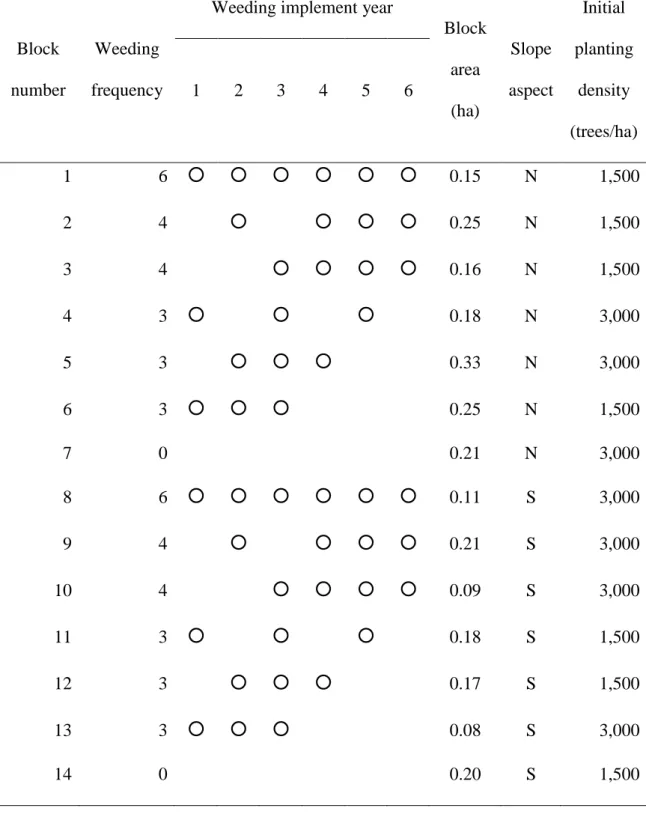
Table 1.1. Timing (years after planting) of weeding, block area, slope aspect and initial planting density. Open circles indicate the implementation of weeding during the indicated year.

Block number

Weeding frequency

Weeding implement year

Block area (ha)

Slope aspect

Initial planting

density (trees/ha)

1 2 3 4 5 6

1 6 ○ ○ ○ ○ ○ ○ 0.15 N 1,500

2 4 ○ ○ ○ ○ 0.25 N 1,500

3 4 ○ ○ ○ ○ 0.16 N 1,500

4 3 ○ ○ ○ 0.18 N 3,000

5 3 ○ ○ ○ 0.33 N 3,000

6 3 ○ ○ ○ 0.25 N 1,500

7 0 0.21 N 3,000

8 6 ○ ○ ○ ○ ○ ○ 0.11 S 3,000

9 4 ○ ○ ○ ○ 0.21 S 3,000

10 4 ○ ○ ○ ○ 0.09 S 3,000

11 3 ○ ○ ○ 0.18 S 1,500

12 3 ○ ○ ○ 0.17 S 1,500

13 3 ○ ○ ○ 0.08 S 3,000

14 0 0.20 S 1,500

8

Chapter 2. The effect of weeding frequency on the mortality and accidental cutting of planted sugi trees.

2.1. Introduction

Recently, several studies have been seeking for a possibility to reduce weeding frequency in Japan, towards low-cost silviculture. These studies discussed reducing of weeding frequency in terms of planted trees growth (Akai et al. 1987; Kinjou et al. 2011a; Hirata et al. 2012; Fukumoto et al. 2015b; Yamagawa et al. 2016) and cost of weeding operation (Kinjou et al. 2011b; Kitahara et al. 2013). However, few studies focused on survival rate of planted trees. It is likely that the survival rate of planted trees decreases by the reduction of weeding frequency. As a result, the number of trees that can be harvested decreases when the survival rate decreases. Thus, we need to clarify relationship between reduction of weeding frequency and survival rate of planted tree.

There are two factors of reducing the tree survival rate. One is the mortality that is caused by competition with weed. For example, Hiraoka et al. (2013) showed that tree mortality of sugi clones was low regardless of weeding operation. This study mainly compared the mortality under the condition of non-weeding and annual weeding, but the effect of reducing the weeding frequency on tree mortality was not quantified. The other factor is accidental cutting caused by human error. Several studies reported that accidental cutting was caused due to low visibility by thick weed (Kinjou et al. 2011a; Ukon and Takeuchi 2011). Yokoi (2001) showed that accidental cutting rate was high when weeding frequency was reduced in Japanese zelkova (Zelkova serrata) stand. Similarly, various studies investigated the relationship between weeding operation and accidental cutting in broad-leaved stand (Maeda 1999; Yokoi et al. 1999). However, few studies clarified the

9

accidental cutting in coniferous stands such as sugi or hinoki (Chamaecyparis obtsusa) stands.

Generally, weed structure such as species composition and weed size depend on slope aspect and initial tree density. Therefore, these factors may affect tree mortality.

Similarly, weed size may affect visibility of weeding operation. Thus, accidental cutting rate was indirectly affected by slope aspect and initial tree density. However, few studies discussed about the effects of slope aspect and initial density on tree mortality and accidental cutting rate under reducing weeding frequency.

In this chapter, we investigated the effects of weeding frequency, slope aspect and initial tree density on rate of tree survival, mortality and accidental cutting. First, we compared mortality rate and accidental cutting rate of 7 years-old sugi saplings with different weeding schedules. Finally, to predict the probability of mortality and accidental cutting in different weeding frequencies, we applied the multinomial logistic regression model using weeding frequency, slope aspect and initial tree density as explanatory variables.

2.2. Materials and Methods Study site and Measurements

The study site was the Takakuma Experimental Forest of Kagoshima University, located on the Osumi Peninsula in southwestern Japan. The details of our study site were referred to the pervious chapter 1. The tree mortality and accidental cutting in study plots were visually confirmed when weeding operation in all study plots had been completed in November, 2012 (Table 2.1, Table Appendix 1, 2). Then, accidental cutting was defined as stem cut off by brush cutter.

10

Data analysis

First, we summarized the descriptive statistics for the effect of weeding frequency, weeding schedule, slope aspect, initial tree density on tree mortality rate and accidental cutting rate using field data. Secondly, we used multinomial regression model to simulate survival rate, mortality rate and accidental cutting rate under different weeding frequency, slope aspect, and initial tree density. The explanatory variables were slope-aspect (NS), initial tree density (D), weeding frequency (F), and each interaction effects (NS×D; NS

×F; D×F). Then, we used the dummy variable that takes a value of 1 if slope aspect was north-facing slope and otherwise, the value 0. Finally, we selected the model on the basis of Akaike’s information criterion (AIC). The selected model was used for prediction of sugi survival, mortality and accidental cutting rate with different weeding frequency.

This statistical analysis was done using the VGAM package in the R 3.1.3 software package (Yee 2010; R Core Team 2014).

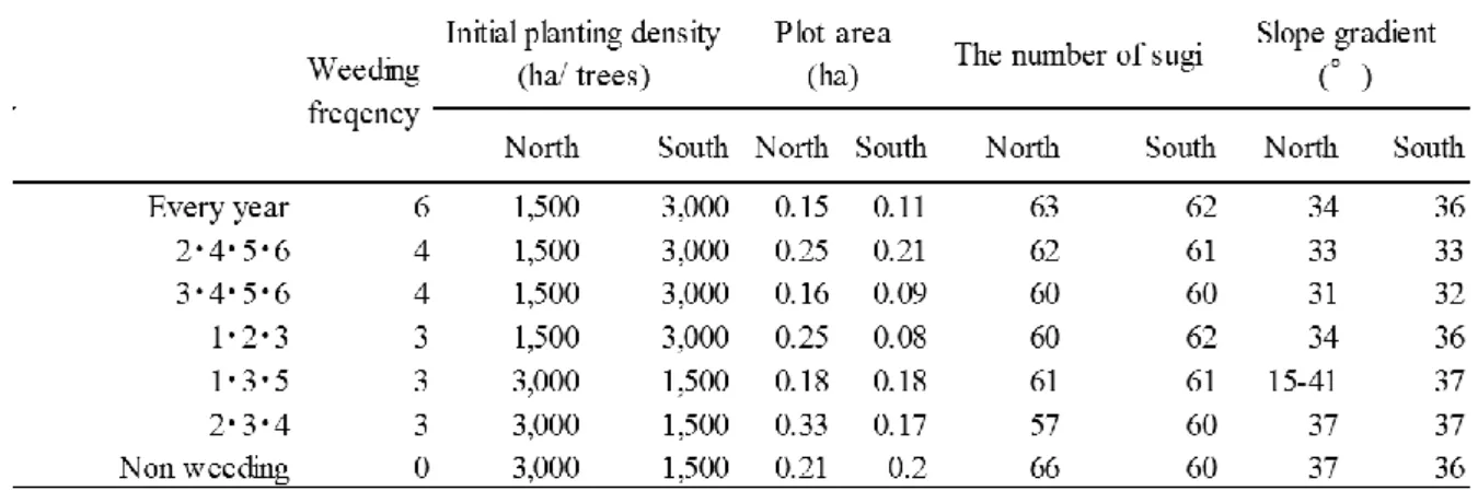
Table 2.1. Summary of study plot and weeding implementation year.

11

2.3. Results

The effect of different weeding frequencies and schedules on sugi mortality and accidental cutting

Figure 2.1 showed that 7 years-old sugi survival, mortality and accidental cutting rate with different slope aspects. On north-facing slope, sugi survival rate was 66.7 –96.8 %.

The sugi mortality rate was the highest when weeding was not conducted. In contrast, the sugi mortality rate was the lowest when weeding was conducted every year. The sugi mortality rate with four-treatment weeding frequency was higher than that of three- treatment weeding frequency, and it was especially high with weeding treatment in years 3, 4, 5 and 6. The sugi mortality with three-treatment weeding frequency was 3.3 %–9.8%, and sugi mortality was especially low with weeding treatment in years 1, 2 and 3. The accidental cutting rate was the highest with weeding treatment in years 3, 4, 5 and 6

Figure 2.1. The 7 years old sugi survival, mortality and accidental cutting rate with different weeding frequency and schedule.

12

(12.1 %). The accidental cutting was also found in three-treatment weeding frequency;

the rate was 1.6 %. The accidental cutting was not found with weeding treatment in every- year or years 1, 2 and 3.

On the south-facing slope, the sugi survival rate was 82.0 –93.3 %. Sugi mortality rate was the highest when weeding was conducted every-year, representing 16.9 %. The sugi mortality rate of the plots except for every-year and in years1, 2 and 3 was 4.9 –8.6 % regardless weeding frequency. The accidental cutting occurred when weeding conducted three and four times; these rate were 6.5 –11.4 %. Both the slope aspects, the accidental cutting did not occur with weeding treatment in every-year or in years 1, 2 and 3. On each slope, the sugi mortality and accidental cutting rate was not found a clear difference between initial planting densities.

The effect of weeding frequency, slope aspect and initial planting density on tree mortality and accidental cutting.

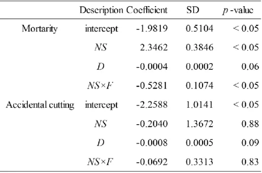
The selected model included NS, D and NS × F (Table 2.2). For mortality, S and NS × F were significant (p <0.05), but not significant (p >0.05) for accidental cutting. D was not significant for both mortality and accidental cutting (p >0.05).

The predicted sugi survival rate on north-facing slope increased with increasing weeding frequency (Figure 2.2). The survival rate of six-treatment weeding frequency on initial tree density of 1,500 (tree/ha) and 3,000 (trees/ha) were 95.3 % and 97.8 %, respectively. In the case of non-weeding, the survival rate for initial tree density 1,500 (trees/ha) and 3,000 (trees/ha) were 55.1 % and 69.5 %, respectively. The predicted mortality rate decreased with increasing weeding frequency, and the mortality rate of six- treatment weeding frequency with the initial tree density 1,500 (trees/ha) and 3,000

13

(tree/ha) were 3.1 % and 1.7 %, respectively. The predicted mortality rate tended to increase when initial tree density was 1,500 (tree/ha). The predicted accidental cutting rate occurred regardless of weeding frequency. On the south facing slope, the sugi survival, mortality and accidental cutting rate were invariable regardless of weeding frequency; the rates were 90.4 %, 6.8 % and 2.7%, respectively. In the case of tree initial density of 3,000 (tree/ha), these rates were 95.2 %, 3.9 % and 0.8 %, respectively.

Table 2.2. Summary of parameters incorporated in the selected model.

14

2.4. Discussion

The sugi mortality varied depending on weeding frequencies, weeding schedules and slope aspects (Figure 2.1). In general, weeding plays an important role for reducing competition of planted trees with weeds for light, soil water and soil nutrients (Wagner et al. 2006). On the one hand, weeds protect planted trees against aridity and high temperature of grand surface (Sakaguchi 1983). One possible reason why slope aspect affected the sugi mortality was the difference of vegetation. For example, pampas grass (Miscanthus sinensis) invaded on south facing slope (Fukumoto et al. 2015b), while broadleaved trees such as pioneer invaded on north facing slope (Kinjou et al. 2011b).

Shigenaga et al. (2012) reported that sugi planted trees growth declined by covered pampas grasses. On the other hand, Tanimoto (1982) reported that sunlight transmitted more through pampas grass stand than broadleaves trees. Therefore, sugi growth was low when weeding was not conducted on south facing slope, because sugi could receive much Figure2.2. Predicted sugi survival rate, mortality rate and accidental cutting rate under different weeding frequency. (a) North-facing slope, (b) South-facing slope.

15

more light in comparison with north facing slope. The mortality rate on south facing slope was higher than that on the north facing slope when weeding was conducted in every year.

Weeding conducted in every year might cause a decline in weed protecting role, and therefore the mortality rate under weeding conducted every year was higher than any other schedules on south facing slope. These results suggest that we should judge suitable weeding frequency and schedule depending on slope aspects.

On north facing slope, the mortality rate was high when weeding was not conducted, and the rate was low when weeding was conducted every year. Additionally, the mortality rate with four-treatment weeding frequency was higher than the three- treatment weeding frequency. These results suggest that the mortality is not always low with more weeding frequency, and the mortality may be affected by weeding schedules.

The sugi mortality rate was high when weeding was conducted only once three years after planting (e.g. treatment in years 3, 4, 5 and 6 or years 2, 4, 5, and 6). This result showed that weeding conducted at least twice in three years after planting is important for reducing tree mortality rate.

The accidental cutting rate was not different among weeding frequency and between different slope aspects. These results suggest that accidental cutting occur a certain number regardless of weeding frequency and slope aspect. However, weeding conducted in every year and in years 1, 2 and 3 did not cause accidental cutting on each slope aspect. Ukon and Takeuchi (2011) reported that weeing conducted during consecutive year could reduce accidental cutting. Therefore, the accidental cutting rate in the plots where weeding conducted consecutive year just after planting was low. On the other hand, the accidental cutting rate was high with weeding treatment in year 3, 4, 5 and 6, because visibility was declined due to invaded weeds. These results suggest that we

16

had better practice weeding during two years after planting to reduce accidental cutting.

The multinomial regression model showed that slope aspect, initial tree density and interaction effect of weeding frequency and slope aspect were selected as significant explanatory variables (Table 2.2). On tree mortality rate, NS × F was significant (p < 0.05).

This result showed that the tree mortality rate for each weeding frequency was different between slope aspects. The tree mortality rate on north-facing slope depends on each weeding frequency (Figure 2.2). Therefore, we have to consider lack of certain amount of planted trees by mortality when weeding frequency is reduced. Yet in south facing slope, the tree mortality was invariable regardless of weeding frequency (Figure 2.2).

Therefore weeding frequency should be reduced in comparison with the conventional weeding frequency. For the accidental cutting rate, all selected variables were not significant (p >0.05) (Table 2.2). Therefore, we conclude that accidental cutting occurs regardless of weeding frequency and slope aspects. In contrast, initial tree density was selected as explanatory variables on tree mortality and accidental cutting model; however, the variables were not significant (p >0.05) (Table 2.2). Nevertheless, predicted sugi mortality and accidental cutting rate under initial planting density 1,500 (trees/ha) were higher than that with 3,000 (trees/ha) (Figure 2.2). Tsutsumi (1994) suggested that replanting is needed when tree mortality rate in the year after planting was more than 20 % for initial tree density of 3,000 (trees/ha) stand. The logistic regression analysis showed that the mortality rate was more than 20 % when weeding was conducted two times or less under 3,000 (trees/ha), or weeding was conducted three times or less for 1,500 (trees/ha). If we follow the suggestion by Tsutsumi (1994), weeding would need at least two times. Furthermore, our result suggested that planted trees mortality and accidental cutting could be reduced if weeding is conducted two times during 3 years after

17

planting.

This chapter focused on the effects of weeding frequency, schedule, slope-aspect and initial plating density on sugi mortality and accidental cutting. In term of mortality rate, we have to consider the optimum weeding schedule depending on slope aspect and initial planting density. The accidental cutting may occur everywhere, and therefore we must be careful for initial setting for the number of trees. On the other hand, our result suggested that sugi mortality and accidental cutting rate increase depending on weeding schedules. The plot where weeding was conducted in years 3, 4, 5 and 6 had high mortality and accidental cutting rates. This result suggests that survival rate significantly decreased when weeding was not conducted two years after planting. Our statistical model could not explain the optimum weeding schedules in terms of sugi mortality and accidental cutting rate. We will have to clarify the optimum weeding schedule taking into account conditions such as slope aspect and initial tree density. Moreover, weeding schedules might affect tree growth and weeding operation time (Wagner et al. 1999;

Kinjou et al. 2011a), and so we will have to comprehensively clarify the effect of weeding schedules on tree growth and operational cost.

18

Chapter 3. The effect of weeding frequency and timing on the height growth of young sugi stands.

3.1. Introduction

Weeding cost reducing is important subject in Japan. Because, weeding cost account approximately 40 % for management cost in early stage. On the other hand, Weeds grow rapidly and may compete with planted saplings without appropriate weeding. As a result, one cannot avoid the growth suppression from weeds when one reduces the number of weeding. Thus, one has to establish a weeding schedule under which the growth suppression from weeds, as well as the number of weeding, is minimized. Several studies have focused on reducing the number of weeding of sugi and hinoki (Akai et al. 1987;

Shimozono et al. 2009; Kinjou et al. 2011a; Hirata et al. 2012; Fukumoto et al. 2015b).

These studies mainly focused on non-weeding or annual weeding, and they showed that the growth of planted trees decreased under the non-weeding (Akai et al. 1987; Hirata et al. 2012). However, the effect of weeding on the growth of planted saplings were not quantified.

Our main objective in this chapter is to investigate the effect of weeding schedules on the height growth of sugi saplings. To achieve this objective, we developed stand-level sugi and weed annual height growth models that accounted for tree spacing, slope aspect, and the prior heights of sugi and weeds. Finally, we simulated sugi height under different weeding scenarios and consistent conditions in terms of tree spacing and slope aspect.

19

3.2. Materials and Methods Study site and Measurements

Our study site was Kagoshima University experimental forests. The detail of description our study site referred to chapter 1. We established study plot included approximately 60 sugi saplings, and measured their heights at the end of each growing season from the first through the sixth growing seasons (i.e., 2007–2012) (Figure Appendix.1, 2). We also measured weed (i.e., broad-leaved trees/shrubs) heights from the first through the sixth growing seasons. For some plots, we randomly selected at least five places and measured the dominant height of weeds in each place from the first through the third year after planting (i.e., 2007–2009). From the four through the sixth growing seasons (i.e., 2010–

2012), we randomly selected 60 places and measured the heights of dominant weeds for all plots. We defined the dominant height as the mean height of the top layer of weeds.

The weeds were measured between late June and early July of the year just before the weeding was conducted.

Data analysis Growth model

A hierarchical Bayesian model was used to determine the stand-level annual height growth of sugi and weeds. We assumed that the observed mean annual sugi and weed height growth of the ith plot in the jth growing season with a normal distribution, as follows:

Gij ~ Normal [ln(𝐺̅_𝑖𝑗) , 𝜎²] (3-1)

where Gij is the observed mean annual height growth of sugi or weeds (m year⁻¹), 𝐺̅_𝑖𝑗 is the expected mean annual height growth (m year⁻¹) of sugi or weeds, and 𝜎² is the

20

variance of the height distribution. The mean annual height growths of sugi and weed were regressed against the explanatory variables, including mean sugi height at the end of prior growing season (H), mean weed height just after weeding (WH), the relative height of weeds to sugi (WHH), slope direction (S), sugi tree spacing (D), and random parameters for each plot. The developed model can be described as:

ln(𝐺̅_𝑖𝑗^𝑐) = 𝛼₀^𝑐+ 𝛼₁^𝑐𝑊𝐻_𝑖𝑗+ 𝛼₂^𝑐𝐻_𝑖𝑗 + 𝛼₃^𝑐𝑊𝐻𝐻_𝑖𝑗+ 𝛼₄^𝑐𝑆_𝑖+ 𝛼₅^𝑐𝐷_𝑖+ 𝜑_𝑖^𝑐 (3-2) ln(𝐺̅_𝑖𝑗^𝑤) = 𝛼₀^𝑤+ 𝛼₁^𝑤𝑊𝐻_𝑖𝑗+ 𝛼₂^𝑤𝐻_𝑖𝑗 + 𝛼^𝑤₃𝑊𝐻𝐻_𝑖𝑗+ 𝛼₄^𝑤𝑆_𝑖+ 𝛼₅^𝑤𝐷_𝑖+ 𝜑_𝑖^𝑤 (3-3) where 𝐺̅_𝑖𝑗^𝑐 is the expected mean annual sugi height growth (m year⁻¹), 𝐺̅_𝑖𝑗^𝑤 is the expected mean annual weed height growth (m year⁻¹), 𝛼₀^𝑐– 𝛼₅^𝑐 and 𝛼₀^𝑤– 𝛼₅^𝑤 are each parameter, and 𝜑_𝑖^𝑐 and 𝜑_𝑖^𝑤 are random parameters for the ith plot. In the case of slope direction, we defined Si as 1 when the slope of the ith plot faced south; otherwise, we assigned Si as 0. We assigned WHij as 0 when the weeding was conducted in the ith plot in the jth growing season. Thus, 𝐺̅_𝑖𝑗^𝑤 was calculated as the growth from 0 m when the weeding was conducted in the ith plot in the jth growing season. WHHij was expressed as WHij divided by Hij.. WHHij was also defined as 0 when the weeding was conducted in the ith plot in the jth growing season. We assigned a normal distribution for the random parameters as follows:

𝜑i ~ Normal [0, 𝜏] (3-4)

where 𝜏 is the variance of 𝜑_𝑖. We assigned a uniform prior to 𝜏, 𝜎² and other parameters (i.e., 𝛼₀– 𝛼₅). To estimate the posterior distributions of the parameters, we used the Markov chain Monte Carlo (MCMC) method using JAGS 3.4.0 software (Plummer 2003) via the rjags package in the R 3.1.3 software package (R Core Team 2014). We obtained posterior samples from four parallel MCMC chains. For each chain, 5,000 samples were obtained with a 50,000-step interval after a burn-in period of 1,000

21

MCMC steps. The Gelman and Rubin 𝑅̂ value was used to confirm the convergence of the MCMC. We set our convergence threshold at 𝑅̂ < 1.1. Model selection was conducted by a backward stepwise procedure from equations (3-2) and (3-3). We selected the model on the basis of the deviance information criterion. We calculated R² from observed and predicted growth of sugi and weeds. Marginal R², which was calculated from fixed factors alone, and conditional R², which was calculated from both the fixed factors and random factors were calculated, since Nakagawa and Schielzeth (2013) recommended.

Weeding simulations

We simulated sugi height after the sixth growing season under the different weeding schedules using the selected model. We assumed that sugi with a 0.6-m height was planted on a slope where site preparation had already been conducted prior to planting (i.e., the initial weed height was 0). These assumptions are based on the common situation of plantation practices in Kagoshima (Shimozono et al. 2009). The simulated weeding frequencies included the (1) non-weeding, and (2) one, (3) two, (4) three, (5) four, (6) five, and (7) six weeding during the six growing seasons. To simulate the weeding schedule, we had several choices regarding the timing of the weeding for each weeding frequency. In this study, we simulated all weeding scenarios for each weeding frequency.

Weeding frequencies of zero, one, two, three, four, five, and six, yield 1, 6, 15, 20, 15, 6, and 1 combinations of their timing, respectively. In total, 64 weeding scenarios were simulated. Then, we used the tree spacing and slope aspect variables if they were included as variables in the selected model. By simulating 64 weeding schedules for their respective slope aspect (i.e., north and south), we ultimately simulated 128 weeding

22

schedules.

We evaluated the influence of weeding frequency on sugi height after six growing seasons, calculating the mean simulated sugi height based on the weeding frequency for the respective slope aspect. To evaluate the importance of the timing of weeding, we simulated sugi height for the three-treatment weeding frequency, because a three-treatment weeding frequency includes more choices (i.e., 20) than the other weeding frequencies. We only simulated tree height on north slopes, because the simulated heights on both slopes showed the same trend.

3.3. Results

Model selection and goodness of fit

Table 3.1. Summary of the parameters for the selected model.

Parameter Description Mean Marginal R² Conditional R²

Sugi model 𝛼₀^𝑐 intercept -0.22 0.72 0.79

𝛼₁^𝑐 WH -0.15

𝛼₂^𝑐 H 0.12

𝛼₃^𝑐 WHH -0.65

𝛼₄^𝑐 S -0.11

𝜎² variance 0.02

Weeds model 𝛼₀^𝑤 intercept 0.38 0.27 0.31

𝛼₂^𝑤 H -0.09

𝛼₃^𝑤 WHH -0.43

𝛼₄^𝑤 S -0.30

𝜎² variance 0.16

WH : mean weed height, H : mean sugi height, WHH : the relative height of weeds to sugi, S : slope direction.

23

All of the model parameters adequately converged (𝑅̂ <1.1). The selected model for sugi included WH, H, WHH, and S (Table 3.1). For weeds, the selected model included H, WHH, and S. D was not selected in either model. The parameter estimates provided a good fit to the observed data. The marginal R² of the sugi and weed models were 0.72 and 0.27, respectively. Similarly, the conditional R² of sugi and weed model were 0.79 and 0.31, respectively.

Weeding scenario

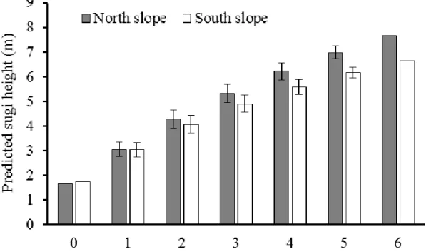
The height of sugi increased with increasing weeding frequency on north- and south- facing slopes (Figure 3.1). Mean sugi height increased by approximately 20 % for every additional weeding. The height when weeding was conducted three times was

Figure 3.1. Summary of the relationship between simulated sugi height and weeding frequency. Error bars indicate standard deviations.

24

approximately 70% of that of the annual weeding.

Sugi height was greatest with weeding treatment in years 1, 2 and 4 (Figure 3.2).

Sugi height was lowest with weeding treatment in years 4, 5 and 6. When the first weeding Figure 3.2. Predicted sugi height under different weeding schedules on three-treatment weeding frequencies in north facing slope.

25

was conducted in the third or fourth growing seasons (e.g., treatment in years 3, 4 and 5 or years 4, 5 and 6), sugi height was shorter than those of the other weeding schedules.

3.4. Discussion

Growth of planted trees is affected by weeds because of competition (Balandier et al.

2005; Kitahara et al. 2013; Hirata et al. 2015). Kitahara et al. (2013) showed that the height growth of planted sugi saplings is suppressed when the apex of the saplings is covered by weeds. This result implies that the relative heights of planted saplings and weeds may explain the interaction between sugi and weeds. Because WHH was selected as an explanatory variable of the model, we confirmed that the relative heights of planted saplings and weeds were important, when selecting weeding schedules. It should be noted that the coefficient of WHH had minus value for weeds model. This may be because the growth of weeds reach its peak after weeds height exceed the height of sugi sapling.

From the simulated results, mean sugi height increased by approximately 20 % for every additional weeding (Figure 3.1). Weeds can continually grow in the absence of weeding. As a result, sugi is suppressed by the continually growing weeds, and sugi height decreas under lower weeding frequencies. For the three-treatment weeding frequency, the sugi height was the highest with weeding treatment in years 1, 2 and 4(Figure 3.2).

Additionally, according to the results of the simulation, sugi height was lowest with weeding treatment in years 4, 5 and 6. These results suggest that the timing of weeding is also important when reducing the weeding frequency. Thus, one has to consider not only the weeding frequency, but also the timing of the weeding, when reducing the weeding frequency. Furthermore, these results imply that earlier weeding is more important than later weeding. Wagner et al. (1999) proposed that weeding immediately after planting

26

yielded better growth of planted trees compared with weeding in later years. Similarly, Mason (2006) reported that weeding in the first year after planting was the most critical for the growth of radiata pine (Pinus radiata) saplings. We also demonstrated that earlier weeding is more important for sugi growth.

The limitation of our model is that the model only considers the relationship between the height of sugi and weeds after weeding. Since the elongation of sugi usually starts before weeding, further study is required to develop the model taking into account the growth before and after weeding. Also, this study only focused on the relationship between the weeding schedule and height growth. However, Kinjou et al. (2011b) showed that the timing of weeding affects the time required for weeding, which was directly linked to its cost. Thus, further study is required to clarify the relationship between weeding schedules and the cost of weeding. Also, the influence of weeding on the growth of diameter and volume should be investigated.

27

Chapter 4. The effect of weeding frequency and timing on weeding operation time.

4.1. Introduction

Weeding is an important practice for sustainable forest management. Weeding aims to reduce competition for light, soil water and soil nutrients between planted trees and other plants. In the case of Japanese forestry, manual treatment using a brush cutter is conducted at least once or twice per year for 5 or 6 years after planting (Tsutsumi 1994). Weed control by means of a brush cutter requires repetitive treatment because of rapid weed regrowth (Biring et al. 2003). This method of weed management results in high costs (e.g.

Dampier et al. 2006; Homagain et al. 2011a). For example, Homagain et al. (2011) reported stand level benefit analysis of 12 vegetation control applied in northern Ontario.

They showed that the aerial herbicide control had the lowest cost (CAD$210.50 ha^-1), repetitive treatment with brush cutter had the highest cost (CAD$1750.00 ha^-1). In the case of Japan, weeding cost accounting for approximately 40% of the total cost during the first 10 years after planting (Yukutake and Yoshimoto 2001). Thus, reduction of the weeding cost is an important objective (Forestry Agency 2016).

Various studies were conducted for the reduction of weeding cost using various approaches in Japan. For example, some studies focused on weeding method (Tange et al.

1993; Ito et al. 2015), weeding treatment season (Itou and Yamada 2001), developing weed prevention seat (Uemura and Taniguchi 2004) and the competition between weed and planted trees (Yamagawa et al. 2016). Especially, many papers focused on the reduction of weeding frequencies (Kinjou et al. 2011a, b; Hirata et al. 2012; Fukumoto et al. 2015b), for example; the growth of planted trees under non-weeding stand (Hirata et

28

al. 2012; Fukumoto et al. 2015) and under some weeding schedules (Kinjou et al. 2011a).

Cost is a key factor for evaluation of treatment choices, because weeding schedules must be as inexpensive as possible. Several studies have focused on the cost of weeding with a brush cutter (e.g. Kinjou et al. 2011b; Kitahara et al. 2013). Kinjou et al.

(2011b) implied that weeding operation time was affected by the height of weeds and the ease with which the operator was able to recognize the planted trees. The authors suggested that the size of planted trees may affect the weeding operation time, because the operator may need to be more careful when the planted trees are small. However, the relationship between the weeding operation time and the weeds’ height and the size of planted trees was not quantified. Similarly, Kitahara et al. (2013) evaluated the relationship between operation time and amount of weeds in a planted forest after the first growing season. The authors suggested that operation time of weeding was affected by the amount of weeds. However, they focused on the stand only just after the first growing season. Given that weeding is conducted for 5 or 6 years after planting, relationships between operation time of weeding and other factors in forests should be evaluated from the first to fifth or sixth growing season. In addition, factors other than the size of weeds and the ease of recognition of the planted trees should be examined. For example, the higher the initial planting density, the more operation time may be required, because operators must circumvent the planted trees. Moreover, slope aspect affects the weeding operation time due to different solar radiation. Weeding is usually conducted in early summer season when we have high temperature and humidity in western Japan. Weeding operation is one of the tough work for operators. The higher solar radiation caused physical exhaustion sever damage for operators; therefore, the factor may affect weeding operation time.

29

The main objective of this chapter was to clarify the effect of weeding frequency and weeding year on the weeding operation time in a sugi stand. To achieve this objective, we developed an operation time model to account for weed height, planted sugi height, slope aspect, initial planting density and relative height of weeds to sugi saplings. We simulated the cumulative operation time under different weeding scenarios and initial planting densities using the developed model.

4.2. Materials and Methods Measurements

Operation time of weeding

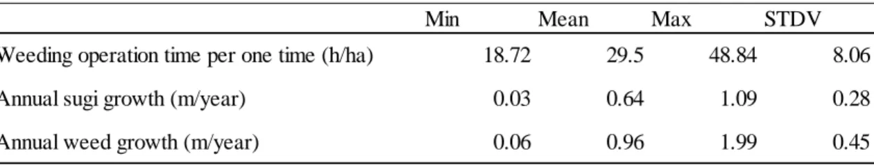
Weeding with a brush cutter was conducted once per year in early July. Three operators worked at each weeding. The same three operators conducted the weeding throughout the six-year experimental period. We recorded operation time during weeding with the brush cutter, excluding the time spent walking into the study blocks, maintaining tools, refueling and taking breaks. The operation time per hectare (h/ha) was calculated for each block area. Given that 23 weeding operations were conducted within each slope aspect (Table 1), in total we recorded operation time data for 46 weeding operations (Figure Appendix 3, 4). The operation time data were summarized in Table 4.1.

Min Mean Max STDV

Weeding operation time per one time (h/ha) 18.72 29.5 48.84 8.06

Annual sugi growth (m/year) 0.03 0.64 1.09 0.28

Annual weed growth (m/year) 0.06 0.96 1.99 0.45

Table 4.1. Summary of field measurements data for weeding operation time (h/ha), annual sugi growth (m/year) and annual weed growth (m/year).

30

Sugi and weed height growth

We measured sugi tree height and weed height around the sugi trees in each plot from the first to the sixth growing seasons (i.e. 2007–2012). The sugi trees were measured after the growing season every year, and weeds were measured before the weeding was conducted. Detailed descriptions of the measurements are provided in chapter 3, we summarized sugi and weed annual height growth (m/year) in Table 4.1. Weed height measurements were not recorded for some plots in some growing seasons. Thus, in this study we used data for 31 weeding operations for which weed height measurements were available.

Data analysis

Operation time model

We used a hierarchical Bayesian model to determine the operation time. We assumed that the observed operation time of the ith plot in the jth implementation of weeding had a normal distribution, as follows:

𝑇_𝑖𝑗~Normal[ln(𝑇̅_𝑖𝑗), 𝜎²] (4-1)

where 𝑇_𝑖𝑗 is the observed operation time per weeding treatment per hectare (h/ha), 𝑇̅_𝑖𝑗 is the expected operation time (h/ha), and 𝜎² is the variance of the operation time distribution. The explanatory variables included weed height (WH), sugi height (H), slope aspect (S), initial planting density (D) and the relative height of weeds to sugi (WHH;

calculated as WH divided by H). WHH was included as an index to express the ease of recognition of sugi. The full model for operation time was expressed as:

ln(𝑇̅_𝑖𝑗) = 𝛼₀+ 𝛼₁𝑊𝐻_𝑖𝑗 + 𝛼₂𝐻_𝑖𝑗 + 𝛼₃𝑊𝐻𝐻_𝑖𝑗 + 𝛼₄𝑆_𝑖 + 𝛼₅𝐷_𝑖𝑗 + 𝜑_𝑖 (4-2)

31

where 𝛼₀~ 𝛼₅ are each parameter, and 𝜑_𝑖 is a random parameter for the ith plot. We assigned a normal distribution for the random parameter as follows:

𝜑i ~ Normal [0, 𝜏] (4-3)

where 𝜏 is the variance of 𝜑i. We assigned a uniform prior to 𝜏 and other parameters.

To estimate the posterior distributions of the parameters, we applied the Markov Chain Monte Carlo (MCMC) method using JAGS 3.4.0 software (Plummer 2003) from within R 3.1.3 software (R Core Team 2014) with the rjags package. We ran four chains each of length 30,000 steps, after burn-in of 1,000 steps and 1/10 thinning. Following previous chapter 3, the Gelman and Rubin 𝑅̂ and deviance information criterion (DIC) were used to confirm the convergence of MCMC and to select the best model, respectively. We calculated the root mean squared error (RMSE) and coefficient of determination (R²) from the observed and predicted operation times. The marginal R² and the conditional R² (Nakagawa and Schielzeth 2013) were also calculated to evaluate the model following chapter 3.

Weeding simulation

We simulated cumulative operation time over the six growing seasons under the different weeding scenarios using the best model. For the simulation, we used the sugi and weed height growth models developed by chapter 2 as follows:

ln(𝐺̅^𝑐) = − 0.22 − 0.15𝑊𝐻 + 0.12𝐻 − 0.65𝑊𝐻𝐻 − 0.11𝑆 (4-4) ln(𝐺̅^𝑤) = 0.38 − 0.09𝐻 − 0.43𝑊𝐻𝐻 − 0.30𝑆 (4-5) where 𝐺̅^𝑐 is the mean annual sugi height growth (m/year), and 𝐺̅^𝑤 is the expected mean annual weed height growth (m/year). Detailed descriptions of the models are provided by chapter 3. Briefly, the explanatory variables include WH, H, WHH and S. The value 1 was

32

assigned to S when the slope faced south; otherwise, zero was assigned. We assumed that initial planted sugi and weed height were 0.6 m and 0 m, respectively, based on our measurements. The simulated weeding frequencies ranged from one to six depending on the weeding treatment during the six growing seasons. We assigned the value zero to WH for estimation of sugi and weed height growth, when the weeding was conducted. For each weeding frequency, there are several options for the weeding year. In this study, we simulated all possible weeding schedules for each weeding frequency. The number of schedules for one, two, three, four, five, and six are 6, 15, 20, 15, 6, and 1, respectively.

In total, there are 63 possible weeding schedules.

We simulated cumulative operation time under the different weeding frequencies under both initial planting densities (i.e. 1,500 and 3,000 trees/ha) on north- and south- facing slopes. Then, Hij and WHij were calculated by the equations (4-3) and (4-4), and we substituted the values in the equation (4-2). We only present simulation results for the north-facing slope, because the simulated operation time on both slopes showed the same trend. To evaluate the effect of the weeding schedules, we focused on the three-treatment weeding frequency, following previous chapter 3. The cumulative operation time and sugi height under both initial planting densities showed the same trend. Thus, we assumed that the initial planting density was 3,000 trees/ha when we focused on the three-treatment weeding frequency.

4.3. Results

Model selection and goodness of fit

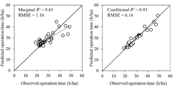
The selected model for weeding operation time included WH, WHH and D (Table 4.2). H and S were not selected in the model. The coefficients of WH, WHH and D had positive

33

values. The marginal R² and RMSE values were 0.65 and 1.10, respectively (Figure 4.1(a)). The conditional R² and RMSE values were 0.93 and 0.18, respectively

Figure 4.1. The relationship between observed operation time and (a) predicted operation time calculated only fixed factor, (b) predicted operation time calculated both fixed and random factors.

2.5% 97.5%

α₀ intercept 2.8310 2.4870 3.2180

α₂ WH 0.1740 0.0784 0.2738

α₃ WHH 0.2056 0.1082 0.3026

α₄ D 0.0001 -0.0001 0.0002

σ² variance 6.81199 Parameter Description Mean

Credible interval

Table 4.2. The summary of posterior distribution and parameter for selected model.

34

Weeding scenario

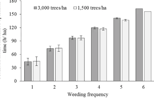
The predicted mean cumulative operation times with annual treatment under initial planting densities of 1,500 and 3,000 trees/ha was 156 and 162 h/ha, respectively (Figure 4.2). The mean cumulative operation time with three-treatment weeding frequency under both initial planting densities was about 97 h/ha. Mean cumulative operation time decreased by approximately 6% for each one-treatment reduction in weeding frequency.

Thus, if the weeding frequency was halved, the cumulative operation time was not halved.

We next focused on the three-treatment weeding frequency. Weeding treatment in years 1, 2, and 6 required the longest operation time, whereas weeding treatment in years 1, 2, and 3 required the shortest operation time (Figure 4.3). The operation time with treatment in years 1, 2, and 6 and that of treatment in years 1, 2, and 3 was 102 and 88 h/ha, respectively. These values represented 63% and 54% of that of the six-year treatment, respectively. The difference in operation time between the two scenarios was 14 h/ha. The operation time required was increased when weeding was not conducted in consecutive years (e.g. treatment in years 1, 2, and 6, or years 1, 3, and 6, or years 1, 5, and 6). In contrast, when weeding was conducted in consecutive years, the cumulative operational time decreased (e.g. treatment in years 1, 2, and 3, or years 2, 3, and 4).

35

Figure 4.2. The predicted cumulative operation time for different weeding frequency under different initial planting density.

36

Figure 4.3. Predicted operation time under different weeding schedules for three-times weeding frequencies.

37

4.4. Discussion

Weeding operation time was affected by WH and WHH (Table 4.2). Given that the coefficients of WH and WHH were positive, the higher the weeds or the higher the weed height relative to sugi height required a longer operation time. The present results confirm the finding by Kinjou et al. (2011b) suggesting that weed height and the ease of recognition of the planted trees affect the weeding operation time. Thus, we conclude that keeping the weed height low is important to reduce the weeding operation time. However, even if the weed height is low, a longer operation time is required if the planted tree height is low; therefore, the planted tree height as well as the weed height is important for reduction of the weeding operation time. The result suggests that the operation time decreases year after year if the weed height is constant, because of the annual tree growth of planted trees.

Initial planting density also positively affected weeding operation time (Table 4.2). One possible reason why initial planting density affects operation time is that operators have to circumvent more planted trees when the planting density is higher.

Recent studies indicate that low-density planting is effective with regard to reduction of the initial planting cost (Sasaki et al. 2009; Ota et al. 2013) and planted tree growth (e.g.

Fukuchi et al. 2011). The present results suggest that reducing the initial planting density promotes reduction of weeding operation time, thus we conclude that low-density planting is also effective for reduction of weeding operation time. However, it should be noted that the reduction in weeding time achieved with low-density planting is much smaller than that attained by reduction of weeding frequency (Figure 4.2).

Cumulative operation time decreased approximately 6% for each one-treatment reduction in weeding frequency. Even if the weeding frequency was halved, the

38

cumulative operation time was not similarly halved (Figure 4.2). When weeding is not conducted in a given year, the operation time for that year is zero. Thus, the cumulative operation time decreased with the reduction of weeding frequency. However, the operation time of weeding is increased in the year immediately following that when weeding is not conducted. This is because WH and WHH increase in the absence of weeding, and have positive effects on the subsequent weeding operation time. Thus, the cumulative operation time does not decline commensurate with the decrease in weeding frequency. Both the operation time reduction due to non-weeding in a given year and the increase in operation time resulting from growth of WH and WHH must be considered.

With a three-treatment weeding frequency, the cumulative operation time tended to increase when weeding was not conducted in consecutive years (e.g. treatment in years 1, 2, and 6, or years 1, 3, and 6, or years 1, 5, and 6) (Figure 4.3). We thus conclude that weeding should be conducted in consecutive years to reduce weeding cost.

This study clarified the factors that affect weeding operation time. We conclude that weeding schedules as well as weeding frequency affect the weeding operation time.

With regard to weeding operation time, we recommend that weeding is conducted in consecutive years. It should be noted that this study only focused on the weeding operation time. Fukumoto et al. (2017) showed that weeding frequency as well as weeding schedule affects the growth of planted trees. Kobe et al. (1995) also indicated that tree mortality is affected by weeding treatment. We expect that the optimal weeding frequency and schedule will be determined by considering not only the cost (i.e. weeding operation time), but also the growth and mortality of planted trees. Thus, additional studies accounting for weeding operation time, growth of planted trees, and planted tree mortality are required. We also have to consider the effect of weeding frequency reduction on total

39

management cost and stand volume for sustainable forest management.

40

Chapter 5. The relationship between sugi height growth and weeding operation time: Assessment of optimal weeding schedules using Monte Carlo method.

5.1. Introduction

The reduction of weeding cost has become important subjects in Japan. Weeding cost can be reduced in principal when weeding is not conducted or when weeding frequency is shortened; however, planted trees growth may be adversely suppressed due to competition with weeds. Therefore, the tendency of negative trend of planted trees growth should be put into consideration when conducting assessment of weeding cost reduction. Some researchers reported about planted trees growth under non-weeding treatment (Hirata et al. 2012, Fukumoto et al. 2015), three-times treatment (Watanabe et al. 2013; Fukumoto et al. 2015a) and various weeding frequency treatment (Kinjou et al. 2011a). For example, Kinjou et al. (2011) showed that sugi height and diameter is decreased as weeding frequency decreases. Hirata et al. (2012) reported that the planted trees height and diameter growth was affected by vertical weed suppressions in non-weeding hinoki stand.

As stated above, several researcher reported about the relationship between weeding frequency reducing and planted trees growth. However, our previous chapter suggested that the sugi height growth is depending not only on weeding frequency but also on weeding schedule. Therefore, we have to clarify the effect of both weeding frequency and schedule on planted trees growth.

Weeding schedules affect not only on planted trees growth, but also on weeding operation time (Watanabe et al. 2013, Fukumoto et al. 2017). For example, Watanabe et al. (2013) reported that cost for weeding conducted for 3 times in years 2, 4 and 6 after

41

planting could reduce approximately only 30 % in comparison with the cost for 6 times of annual weeding treatment. This result indicated that weeding cost is not necessarily proportional to weeding frequency.

Although the importance of weeding schedule for decision of optimum weeding schedules is clarified in the previous chapters, there is no study that discusses the optimum weeding schedules in terms of sugi height and weeding operation time. Therefore, to decide the optimum weeding schedules, it is necessary to clarify the relationship between sugi height and operation time. The main objectives in this chapter are to clarify the relationship between sugi height growth and weeding operation time, and then to propose optimal weeding schedules by applying Monte Charlo method.

5.2. Materials and Methods Data collection

We applied field measurements data, which were obtained from our study site. The data included the sugi mean height (m), weed mean height (m) and weeding operation time per one time (h/ha) for a 6 year-period after planting in each blocks (Table 4.1). The description of field measurements method and data described chapter 3 (sugi and weed height) and 4 (weeding operation time).

Statistical model

We assumed that the observed mean annual sugi and weed height growth with a normal distribution, as follows:

𝐺^𝑐~ Normal [ln(𝐺̅^𝑐) , 0.02] (5-1) 𝐺^𝑤~ Normal [ln(𝐺̅^𝑤) , 0.16] (5-2)

42

𝑇~Normal[ln(𝑇̅), 6.81] (5-3)

where 𝐺 is the observed mean annual height growth of sugi or weeds (m year⁻¹), 𝐺̅ is the expected mean annual height growth (m year⁻¹) of sugi or weeds, and T is the observed operation time per weeding treatment per hectare (h/ha), 𝑇̅ is the expected operation time (h/ha). 0.02, 0.16 and 6.81 indicates the variances. The statistical models are summarized in the chapters 3 and 4. The expected mean annual height growth and the expected operation time per one time as follows;

ln(𝐺̅^𝑐) = − 0.22 − 0.15𝑊𝐻 + 0.12𝐻 − 0.65𝑊𝐻𝐻 − 0.11𝑆 （5-4）

ln(𝐺̅^𝑤) = 0.38 − 0.09𝐻 − 0.43𝑊𝐻𝐻 − 0.30𝑆 （5-5） ln(𝑇̅) = 2.8310 + 0.1740𝑊𝐻 + 0.2056𝑊𝐻𝐻 + 0.0001𝐷 （5-6）

where 𝐺̅^𝑐 is expected mean annual sugi height growth (m/ year), 𝐺̅^𝑤 (m/ year) is expected mean annual weed height growth (m/ year) and 𝑇̅ is expected operation time per one time (h/ ha). The explanatory variables includes the mean sugi height prior growing seasons(𝐻) (m), weed height just after weeding operation (𝑊𝐻) (m), relative height weed to sugi (WHH), slope aspect (𝑆) and tree initial planting density (𝐷) (trees/

ha). Then, 𝑊𝐻𝐻 was expressed as 𝑊𝐻 divide by 𝐻. In the case of slope aspects, we defined S as 1 when the plot faced south, otherwise 0.

Data analysis

To clarify the relationship between sugi mean height and weeding operation time, we simulated 6-years old sugi height and cumulative weeding operation time under different weeding frequencies and schedules. In total, we simulated 64 weeding schedules. Mean annual height growths and operation time per one time were randomly generated from equation (5-4), (5-5) and (5-6). Then, we repeated 100 times sugi height and weeding