東北大学機関リポジトリTOUR

climbing-over, tipping-over, and sliding-down

conditions

著者

Ryosuke Yajima, Keiji Nagatani, Yasuhisa

Hirata

journal or

publication title

Advanced Robotics

volume

33

page range

1060-1071

year

2019-09-24

URL

http://hdl.handle.net/10097/00129147

To appear in Advanced Robotics Vol. 00, No. 00, January 2019, 1–28

Full Paper

Research on traversability of tracked vehicle on slope with unfixed obstacles: Derivation of climbing-over, tipping-over, and sliding-down conditions

Ryosuke Yajimaa∗ _{, Keiji Nagatani}b_{, and Yasuhisa Hirata}a_.

a_{Graduate School of Engineering, Tohoku University, Sendai, Miyagi, Japan;}b_{New Industry Creation} Hatchery Center, Tohoku University, Sendai, Miyagi, Japan

(v1.0 released January 2019)

When a tracked robot explores a volcanic environment, it faces difficulty in climbing over unfixed obstacles such as loose rocks on the ground. Such unfixed obstacles sometimes cause the sliding-down or tipping-over of the robot. Although such phenomena should be avoided for the success of the mission, they have not been sufficiently studied yet. Therefore, this research aims at understanding the phenomena for a tracked vehicle climbing an unfixed obstacle on a slope, and considers the conditions of climbing-over, tipping-over, and sliding-down. To simplify the problem, a model of a single track and circular-cross-section obstacle is used in this research. The climbing-over and tipping-over conditions are derived from the geometric relationship, and the sliding-down condition is derived from statics. Moreover, some experiments using an actual robot are conducted to verify the validity of the conditions. The results show that the derived conditions are reasonable. Furthermore, it is revealed that unfixed obstacles typically tend to slide down more than fixed obstacles because of the number of contact points that can support a robot.

Keywords: Tracked robot; Obstacle climbing; Unfixed obstacle; Volcano exploration

1. Introduction

Japan has 111 active volcanoes, or approximately 7 % of all active volcanoes in the world. When active volcanoes erupt, various phenomena occur, leading to disasters such as cinder or ash fall, pyroclastic flow, lava flow, debris flow, the collapse of volcanic edifices, and volcanic gas. Damages caused by these disasters are also various and include direct damage by pyroclastic flow for a short time and economic damage that affects traffic and agriculture for a long time. Japan has suffered such damage in the past. For example, since the Heisei period, Mt. Unzen erupted in 1991 and 47 people were left dead or missing by the pyroclastic flow [1]. In 2014, Mt. Ontake erupted and 60 people were left dead or missing by cinder, etc. [2]. Such volcanic phenomena will be difficult to avoid in the future; therefore, actions toward disaster prevention or mitigation are essential.

An important issue with regard to volcanic disaster prevention or mitigation is the observation of active volcanoes. In Japan, 50 volcanoes were chosen by the coordinating committee for the prediction of volcanic eruption [3]. To obtain premonitory phenomena of the 50 volcanoes, volcanic observation devices such as seismometers and telephotographic cameras were installed for 24-hour observation. However, these devices cannot observe eruptions from unexpected places because they are stationary devices. In addition, volcanic eruptions may damage the devices, particularly those close to the craters. However, it is difficult for humans to reinstall such devices

directly because of restricted areas around the crater when an active volcano erupts. Therefore, robots are being researched and developed to observe volcanic environments instead of humans [4].

There are suitable locomotion types of observation robots according to purpose. For example, flying robots are useful for rapid observation in a wide area [5–8]. Conversely, surface moving robots are useful for long-term observation or detailed observation of the ground. This type includes walking robots [9, 10], wheeled robots [11–14], and tracked robots. However, walking robots are typically complex, and their moving speed is very slow. Wheeled robots, particularly small-sized wheeled robots, have problems in that their traversability on slopes and uneven terrain is not high. Therefore, tracked robots are suitable as volcano exploration robots because they have high traversability on slopes and uneven terrain, and they have a simple structure. Actually, some tracked-type volcano exploration robots have been developed and evaluated in volcanic areas [15–18].

In conventional research related to tracked robots in volcanic environments, traversability on weak-soil slopes was examined [19, 20]. This is because robots face locomotion problems such as slipping and sticking because of volcanic ash and small lapilli on the slope. However, in reality, when tracked robots move in a volcanic environment, it is also necessary to climb over rocks that are the same size or larger than the robots. Actually, in field tests with the tracked robot ”Quince” at Mt. Aso in 2013, there were various large and small rocks on the ground. When Quince climbed a rock, sometimes it succeeded in climbing over. However, sometimes it failed to climb owing to the rolling of loose rocks (Figure 1).

[Figure 1 about here.]

Based on the field tests, we consider that the ability of a robot to climb is related to the state of the obstacles. Obstacles in volcanic environments can be roughly divided into two types.

I Obstacles that are fixed on the ground and are not moved by the robot’s force, such as the roughness of the ground and buried rocks.

II Obstacles that are not fixed on the ground and may be moved by the robot’s force, such as loose rocks on the ground.

In this study, I and II are defined as ”fixed obstacles” and ”unfixed obstacles,” respectively. For fixed obstacles, the prediction and improvement of the traversal performance on steps and stairs for tracked robots have been researched. For example, a stair-climbing motion was divided into some sub-motions and analyzed based on dynamics. Then, a climbing assessment method and tip-over prediction algorithm were proposed [21–24]. Moretip-over, in research for step climbing, Rajabi et al. [25] analyzed climbing conditions based on geometry and predicted the height of the step that the robot can climb over at relatively high accuracy. An example of a volcanic environment is the blade-type crawler mechanism created by Yamada et al [18]. In this research, the climbing performance on steps, including the effect of blades on tracks, was analyzed and verified for fixed obstacles. Conversely, unfixed obstacles have not been sufficiently studied although phenomena leading to mission failure, such as sliding-down and tipping-over, may occur.

Therefore, the objective of this research is (1) to understand phenomena that occur when a tracked robot climbs an unfixed obstacle and (2) to improve the climbing performance of tracked robots on unfixed obstacles. In this paper, we focus on the former, and the occurrence conditions of the phenomena are derived and verified. This paper is organized as follows. Section 2 describes the research scope and targets. Section 3 derives the climbing-over, tipping-over, and sliding-down conditions of tracked robots. In section 4, each derived condition is verified by experiments. Finally, section 5 discusses the difference between fixed and unfixed obstacles, and methods to improve the climbing performance.

2. Research scope 2.1 Target phenomena

The phenomena dealt with in this research are as follows when a tracked robot climbs an obstacle on a slope:

Climbing-over

The center of gravity of the tracked robot passes over an obstacle, and the front end of the robot falls forward.

Tipping-over

The center of gravity of the tracked robot does not pass over an obstacle, and the robot turns upside down.

Sliding-down

A tracked robot slides downward on a slope.

This research aims to reveal the occurrence conditions of the above phenomena and the differ-ences between fixed and unfixed obstacles on a slope.

2.2 Target robot, obstacle, and environment

Typically, a volcanic environment is an uneven slope. The ground is sometimes compacted and sometimes weak. Rocks as obstacles also have various sizes and shapes. Moreover, a tracked robot is sometimes required to climb a slope vertically and sometimes to traverse a slope horizontally. Actual environments and conditions are so complex, as shown in the above, that the target environment is defined as follows to simplify the problem:

The target environment consists of a tracked robot, a constant slope, and a fixed/unfixed obstacle. This research deals with a situation when a tracked robot is on top of the obstacle over an inclined slope shown in Figure 2. The robot’s locomotion direction is along the inclination direction of the slope, where a two-dimensional side view plane is only considered. Although we have confirmed that the tracked robot with a simple-arc shape on the front of the wheel can climb on top of the cylindrical obstacles to a certain extent from preliminary experiments, the dynamics when the robot moves from the sloped surface to on top of the obstacle is not treated in this study. From this assumption, any shape can be applied to the front section of the wheel. There are numerous studies regarding the robot’s climbing dynamics from the ground to fixed obstacles [21, 26–28]. However, the unfixed obstacle with a single degree of freedom along the robot’s locomotion direction is not examined in previous studies. The robot’s climbing dynamics from the ground to unfixed obstacles should be more complex than fixed obstacles because an obstacle could move when a robot pushes it. The details of the target robot, slope, and obstacle are as follows:

Tracked robot

The target robot is a single tracked robot. In recent years, to improve the traversability, there have been many tracked robots with sub-tracks [29–31]. However, in this research, sub-tracks are not considered. In addition, the robot has no patterns such as grousers on the surface of the track belt.

Slope

The target slope is flat and solid. Although ground with weak soil and obstacles exists in actual volcanic environments [32], it is not dealt with here.

Obstacle

The target obstacle is a cylindrical obstacle lying in a rolling direction on the slope. There are two conditions: fixed and unfixed. Although a typical unfixed cylindrical obstacle can-not maintain its position because of its rolling, in this research, it is assumed that it maintains its position until the robot climbs on it.

[Figure 2 about here.]

3. Derivation of climbing-over, tipping-over, and sliding-down conditions 3.1 Definition of model and parameters

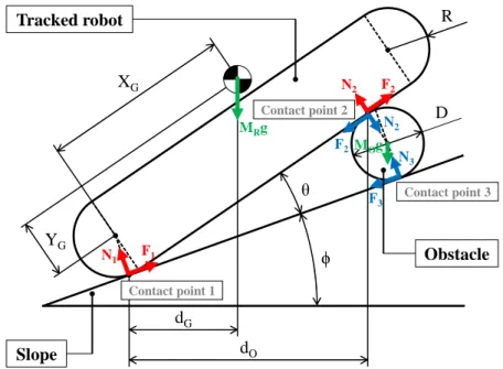
First, the model and parameters are defined. Figure 2 shows a model of the targets in a two-dimensional plane.

The centroid position of the robot is represented as XG and YG. R denotes the track radius

of the front end and rear end of the robot, and MR denotes the mass of the robot. The angle

between the robot and the slope is represented as θ. The slope angle is ϕ. In addition, the cylindrical obstacle has a diameter of D. The mass of the obstacle is MO, and it is assumed that

its center of gravity matches the circle’s center of the cross section. Each contact point is defined as follows:

Contact point 1: The contact point between the robot and slope Contact point 2: The contact point between the robot and obstacle Contact point 3: The contact point between the obstacle and slope

The normal force, frictional force, and coefficients of static friction at each contact point are represented as Ni, Fi, and µi, respectively. Here, the index i is the above number of corresponding

contact points: 1, 2, or 3. g is the acceleration of gravity.

3.2 Climbing-over condition

As described above, Rajabi et al. [25] derived the geometric climbing condition for a tracked robot climbing a step on flat ground. In this research, Rajabi’s method is applied to a tracked robot climbing a fixed/unfixed obstacle on a slope.

This method is based on the idea that a tracked robot can climb over an obstacle when the center of gravity of the robot reaches just above contact point 2. This can be expressed as follows:

dG= dO (1)

where dG is the horizontal distance from contact point 1 to the center of gravity of the robot,

and dO is the horizontal distance from contact point 1 to contact point 2. These are expressed

as follows:

dG= XGcos (θ + ϕ)− YGsin (θ + ϕ)− R sin ϕ (2a)

dO = { R tanθ 2 + D 2 (1 + cos θ) tan θ − D 2 (1 + cos θ) tan ϕ } cos ϕ (2b)

There are two differences between the step on flat ground and the cylindrical obstacle on a slope, as follows:

1) Contact point 1 changes according to the slope angle, and not just under the rear axis of the robot.

2) Contact point 2 moves when a robot moves forward owing to the circular cross section. When the robot climbs over the obstacle, the angle θ between the robot and the slope is derived by substituting the slope angle ϕ and the obstacle diameter D into Equations (2a) and

(2b) and solving Equation (1). Furthermore, by changing the values of ϕ and D, the climbing-over condition is represented by a curved surface, as shown in Figure 3(a). In this graph, the x-axis represents the slope angle ϕ, the y-axis represents the obstacle diameter D, and the z-axis represents the angle θ between the robot and the slope. This graph indicates that when the robot climbs an obstacle with a diameter D on slope ϕ, the robot can climb over the obstacle at the angle θ. Moreover, as seen from the positive part of the z-axis, there is an area that does not exist the curved surface (Figure 3(a)). This indicates that the robot cannot climb over under the combinations of ϕ and D in this area.

When the condition is satisfied, the rear end of the robot is going to leave the slope in case of an unfixed obstacle, as with the case of a fixed obstacle. However, the robot cannot climb over it. When the rear end of the robot leaves the slope, contact point 2 carries the entire weight of the robot, and the force on contact point 2 rolls the obstacle downward of the slope. Then, the robot slides down. To avoid the above phenomenon, the position of contact point 2 should be moved forward. However, the single tracked robot cannot change the position of contact point 2 arbitrarily. Thus, the robot never climbs over an unfixed obstacle.

3.3 Tipping-over condition

The tipping-over condition is derived from the geometric relationship between the center of gravity of the robot and the contact point of the robot on the slope. While the robot moves forward, it tips over when the center of gravity of the robot reaches just above contact point 1. Therefore, the tipping-over condition can be expressed as the following equation by using the distance dG (Equation (2a)):

dG= 0 (3)

The angle θ between the robot and the slope at the moment of tipping-over is derived by substituting the slope angle ϕ into Equation (3). This is determined regardless of the obstacle diameter D. Then, as shown in Figure 3(b), various tipping-over conditions can be derived by changing values of ϕ. The meaning of the graph and the axes is the same as the climbing-over condition.

It is thought that the tipping-over condition can be applied not only to fixed obstacles but also unfixed obstacles because this condition is determined by only the state of the robot.

3.4 Sliding-down condition

As the frictional forces at each contact point are deeply related to the sliding-down condition, it is assumed that the robot’s motion is quasi-static and the condition is considered based on statics. Furthermore, as the state of the obstacle affects, each condition of fixed and unfixed obstacles is derived individually.

3.4.1 Fixed obstacle

In the case of a fixed obstacle, whether the robot keeps its posture without sliding-down is determined by only whether the equilibrium of forces and moments of force acting on the robot can be maintained. This equilibrium is expressed by the following equations:

F1− N2sin θ + F2cos θ = MR· g · sin ϕ (4a)

N2LN2+ F2LF2 = MR· g · LG (4c)

where LN2, LF2, and LG in Equation (4c) represents the distances from contact point 1 to the

line of action of each force N2, F2, and MR· g, respectively. The parameters are expressed as

follows: LN2 = D 2 (1 + cos θ) sin θ − R tan θ 2 + R sin θ (5a) LF2 = R (1− cos θ) (5b)

LG= dG= XGcos (θ + ϕ)− YGsin (θ + ϕ)− R sin ϕ (5c)

Here, one case of the sliding-down condition is considered. When the robot moves forward, the frictional force at contact point 1 reaches the maximum static friction force. However, the sliding-down phenomenon does not occur yet because the robot is supported by contact point 2. When the robot moves farther forward, frictional forces at both contact points 1 and 2 reach the maximum static friction force. At this moment, the equilibrium cannot be maintained, and the robot starts sliding down. The same phenomenon occurs when the reaching order of the maximum static friction force at each contact point is reversed. Conversely, the sliding-down phenomenon does not occur when the frictional force does not reach the maximum static friction force.

When the frictional force reaches the maximum static friction force, the following equation is established:

Fi= µi· Ni (6)

The angle θ between the robot and the slope, and the normal force N1 and N2 at the moment

of sliding-down, are derived by substituting the slope angle ϕ, obstacle diameter D, and Equa-tion (6) into EquaEqua-tion (4). Then, as shown in Figure 3(c), the sliding-down condiEqua-tion for fixed obstacles can be derived by changing the values of ϕ and D. The meaning of the graph and the axes is the same as other conditions.

3.4.2 Unfixed obstacle

In the case of an unfixed obstacle, the force acting on the obstacle should be considered. The equilibrium of forces and moments of force acting on the robot are the same as in the above Equation (4). The equilibrium of forces and moments of force acting on the obstacle are expressed as follows:

N2sin θ− F2cos θ− F3 = MO· g · sin ϕ (7a)

−N2cos θ− F2sin θ + N3= MO· g · cos ϕ (7b)

F2· D

2 = F3· D

2 (7c)

The normal force Ni and frictional force Fi at each contact point are derived by solving

simul-taneous Equations of (4) and (7).

Here, one case of the sliding-down condition is considered. When the robot moves forward, the frictional force at contact point 1 reaches the maximum static friction force. When the

robot moves farther forward, the obstacle starts moving because it is not fixed on the slope, and the robot cannot keep its posture. At this moment, because contact point 1 cannot produce a larger force, the robot slides down, and the obstacle rolls down. Conversely, the sliding-down phenomenon does not occur when the frictional force does not reach the maximum static friction force.

The angle θ between the robot and the slope at the moment of sliding-down is derived by substituting the slope angle ϕ and obstacle diameters D, N1, and F1, which are derived from

simultaneous Equations of (4) and (7), into the Equation (6). Then, as shown in Figure 3(d), the sliding-down condition for unfixed obstacles can be derived by changing the values of ϕ and D. The meaning of the graph and the axes is the same as other conditions.

3.5 Integration of three conditions

According to the previous sections, all conditions are represented by the slope angle ϕ, obstacle diameter D, and the angle θ between the robot and the slope. Therefore, Figure 4(a) is obtained by integrating all of the conditions. This graph indicates that each phenomenon occurs at an angle θ when the robot climbs an obstacle with a diameter D on a slope with an angle ϕ. However, one phenomenon in which angle θ is the minimum value can be observed. This is because the angle θ increases from the initial angle θ0 gradually while it overcomes the obstacle. Therefore,

Figure 4(b) shows the actual phenomenon obtained by maintaining the lowest angle θ. Here, the initial angle θ0 is the angle between the robot and the slope when the front end of the robot ride

on the obstacle, and this is expressed as follows:

θ0= 2 tan−1 ( −L +√L2_{+ 2RD} 2R ) (8)

[Figure 3 about here.] [Figure 4 about here.]

4. Experimental verification of conditions 4.1 Experiment description

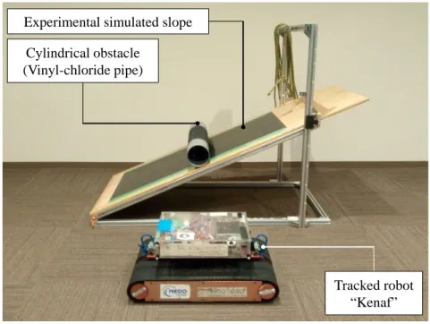
Obstacle-climbing experiments using a real tracked robot were conducted to verify the validity of the conditions described in section 3. In this experiment, a tracked robot climbs a cylindrical obstacle lying in a rolling direction on a slope. During the motion, the behavior and angle θ between the robot and the slope are observed. The angle θ is measured by using the inertial measurement unit (IMU) equipped on the robot. The slope angle ϕ, obstacle diameter D, ob-stacle’s fixed/unfixed condition were changed, and three trials were conducted using each set of conditions. The phenomenon that occurred more frequently was recorded as the result of a set. The details of the robot, slope, and obstacle are described in the following text:

Tracked robot

Tracked robot ”Kenaf” was used as the target robot in this experiment (Figure 5). Although a typical Kenaf has four sub-tracks, only two main tracks were used in this experiment. The track belts were flat without grousers. Table 1 lists the specifications of the Kenaf that are necessary to derive the conditions. The moving speed was set at a sufficiently slow speed of 0.05 m/s.

Slope

A simulated artificial slope was used as the target slope (Figure 5). This slope consisted of aluminum frames and a plywood board, and the slope angle could be finely adjusted. A nitrile rubber sheet was put on the surface of the plywood board to reduce the slippage of the robot. Moreover, there were fixing holes on the surface to reproduce a fixed obstacle.

Obstacle

Vinyl chloride pipes were used as the target obstacles (Fig. 5), and nonslip tape coated with mineral particles was put on the surface of the pipes to reduce slippage. The length of the pipes was 200 mm longer than the width of the robot. The diameters of the obstacles were 33, 61, 90, 115, 141, and 166 mm. Moreover, there were fixing holes on the surface of the obstacle to reproduce a fixed obstacle.

[Figure 5 about here.]

4.2 Climbing-over, tipping-over, and sliding-down conditions of Kenaf

Curved surfaces of Figures 6 and 10 show each condition when Kenaf climbs fixed and unfixed obstacles, derived by the method shown in section 3. The x-axis represents the slope angle ϕ, the y-axis represents the obstacle diameter D, and the z-axis represents the angle θ between the robot and the slope. In addition, Table 2 shows the coefficients of static friction at each contact point.

In the case of fixed obstacles, the climbing-over condition crosses the sliding-down condition. When the target obstacle is small, Kenaf can climb over it. When the target obstacle is large, Kenaf slides down. Conversely, in the case of unfixed obstacles, the sliding-down condition is always under the climbing-over condition. This indicates that Kenaf is not going to climb over obstacles because sliding-down is dominant.

[Table 1 about here.] [Table 2 about here.]

4.3 Experimental results 4.3.1 Fixed obstacles

The results of fixed obstacles are summarized in Figure 6. In this graph, points that indicate the results are plotted in a graph of conditions. The angle θ at which climbing-over and sliding-down occurred in the experiments is the maximum value of the angle θ. This is because the angle θ increases gradually when a robot moves forward on the obstacle, and it decreases when the robot climbs over or slides down. Furthermore, in the case of tipping-over, because the angle θ just increases and it is difficult to discriminate tipping-over, the angle θ is defined as the value derived from Equation 3.

As shown in Figure 6, the results correspond approximately to each condition. Therefore, the derived conditions for fixed obstacles are reasonable. In the experiments, when the center of gravity of Kenaf reached just above the contact point between Kenaf and the obstacle, Kenaf fell forward and climbed over (Figure 7). When the angle θ reached the sliding-down condition, Kenaf slid down (Figure 8). Sometimes, according to the conditions, the sliding-down-distance was short and the robot stayed in one place. In addition, Kenaf tipped over generally when the angle θ reached the tipping-over condition (Figure 9). However, sometimes sliding-down occurred in the vicinity of the boundary between the tipping-over and sliding-down conditions because the surface state of the track belt, the slope, and the obstacle was not uniform, and the coefficients

of the static friction had errors.

[Figure 6 about here.] [Figure 7 about here.] [Figure 8 about here.] [Figure 9 about here.] 4.3.2 Unfixed obstacle

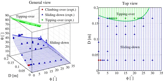
The results for unfixed obstacles are summarized in Figure 10. The angle θ at which each phenomenon occurred in the experiments is the same as that of the fixed obstacles.

As shown in Figure 10, the results correspond approximately to each condition. Therefore, the derived conditions for unfixed obstacles are also reasonable. As with the case of fixed obstacles, in the experiments, when the center of gravity of Kenaf reached just above the contact point between Kenaf and the slope, Kenaf tipped over (Figure 13). Conversely, unlike the case of fixed obstacles, the obstacle rolled and Kenaf slid down largely when sliding-down occurred because the obstacle was not fixed on a slope (Figure 12). Moreover, although it is expected that sliding-down occurs when the slope angle ϕ and the obstacle diameter D are small, Kenaf climbed over the obstacle (Figure 11). It is considered that this is because quasi-static are assumed in the derivation of conditions, but the actual robot’s motion was dynamic. In particular, when the slope angle ϕ and the obstacle diameter D are small, the climbing-over and sliding-down conditions are close. For this reason, it is assumed that the robot climbs over before the robot slides down drastically owing to the influence of the robot’s speed. Furthermore, in the vicinity of the boundary between the climbing-over condition and the sliding-down condition, although the rear end of Kenaf left the slope and Kenaf was about to climb over, it finally slid down.

[Figure 10 about here.] [Figure 11 about here.] [Figure 12 about here.] [Figure 13 about here.]

5. Discussion

5.1 Difference between fixed and unfixed obstacles

As described in section 3, the difference between the fixed and unfixed obstacles is the sliding-down condition. Whether the robot slides sliding-down depends on whether the frictional forces to maintain the posture of the robot can be generated. In the case of unfixed obstacles, only the frictional force of contact point 1 between the robot and the slope affected the sliding-down because the obstacle could be rolled. Conversely, fixed obstacles can be regarded as part of the slope because they cannot be moved. Therefore, the frictional forces of not only contact point 1 between the robot and the slope but also contact point 2 between the robot and the obstacle affect the sliding-down phenomenon. This difference, whereby a robot has either one or two supporting points, changes the tendency of the sliding-down of the robot. Unless the coefficients of static friction are extremely low, an unfixed obstacle with one supporting point more easily

causes sliding-down than a fixed obstacle with two supporting points. As a result, an unfixed obstacle is very difficult for a robot to climb over.

5.2 Improvements to obstacle climbing performance

Considering the above, it is thought that there are some approaches to make a robot climb over a larger unfixed obstacle on a steeper slope.

First, because fixed obstacles are more difficult to cause sliding-down, changing unfixed obsta-cles to fixed obstaobsta-cles by fixing them on a slope is one idea. Driving in piles and binding with an adhesive or a resin may be effective. For example, a study by Napp et al. [33] can be applied. Furthermore, fixing an obstacle to a track belt of the robot may also be effective. In this case, it can be regarded as part of the robot, and the robot is supported by contact point 1 between the robot and the slope and contact point 3 between the obstacle and the slope. Devising track belts can be considered an idea for this. For example, obstacles are partly bound by using flexible materials that follow their shape [34] and grousers that catch them [21, 22].

Second, there is a possibility that the climbing performance can be improved by optimally controlling the angle θ, the position of contact point 2 between the robot and the obstacle, and the centroid position of the robot which affect to occurring each phenomenon. The sub-tracks described in section 2 can be effective in controlling them. However, this method may worsen the climbing performance according to the sub-track angles. It is necessary to reveal the relationship between the sub-tracks and each condition, and to work out the optimal motion strategy of the sub-tracks.

Third, from the experimental results for unfixed obstacles, speeding up the robot may also improve the climbing performance. Intuitively, it can be assumed that the faster the robot, the higher the climbing performance. To predict the climbing performance accurately and to control the speed optimally, the occurrence conditions of each phenomenon considering the dynamics are required.

6. Conclusion

When a tracked robot climbs over an unfixed cylindrical obstacle on a slope, in this research, the climbing-over, tipping-over, and sliding-down conditions were derived for a single tracked robot. The climbing-over and tipping-over conditions were derived from the geometric relationship. By contrast, the sliding-down condition was derived from statics. The conditions were verified by indoor experiments using both fixed and unfixed obstacles. The results showed that the derived conditions were reasonable. Moreover, it was observed that the difference between fixed and unfixed obstacles is a tendency of the sliding-down phenomena. The reason is that in the case of fixed obstacles, the frictional forces of not only the contact point between the robot and the slope but also the contact point between the robot and the obstacle affect the sliding-down phenomenon because the obstacle can be regarded as part of the slope. Conversely, in the case of an unfixed obstacle, only the frictional forces of the contact point between the robot and the slope affect the phenomenon because the obstacle can be moved.

Future work is divided roughly into two topics: to expand the conditions and to apply this to improve the climbing performance. The former includes experiments under different conditions such as other shapes of obstacles including ellipses, polygons, and more complex shapes such as actual rocks. Although the phenomena were considered in a two-dimensional plane in this paper, it is necessary to expand to three-dimensional space when a robot traverses a slope. Moreover, a discussion of the conditions considering the dynamics is also required to improve the accuracy of the conditions. The latter reveals the influence of sub-tracks and the optimal motion strategy of sub-tracks. Patterns such as grousers on the surface of the track belt will also be studied.

phenomena of the robot will be understood accurately, and optimal design and control methods for tracked robots will be obtained. Furthermore, tracked robots will be able to move stably in environments with unfixed obstacles, and more reliable volcano exploration will be realized.

References

[1] Setsuya Nakada and Toshitsugu Fujii. Preliminary report on the activity at Unzen Volcano (Japan), November 1990-November 1991: Dacite lava domes and pyroclastic flows. J. Volcanol. Geotherm. Res., 54:319–333, 1993.

[2] Takayuki Kaneko, Fukashi Maeno, and Setsuya Nakada. 2014 Mount Ontake eruption: Characteris-tics of the phreatic eruption as inferred from aerial observations the Phreatic Eruption of Mt. Ontake Volcano in 2014 5. Volcanology. Earth, Planets Sp., 68(1):72, 2016.

[3] Japan Meteorological Agency. Monitoring of Earthquakes, Tsunamis and Volcanic Activity. [4] Keiji Nagatani. Recent trends and issues of volcanic disaster response with mobile robots. J. Robot.

Mechatronics, 26(4):436–441, 2014.

[5] Akira Sato. The RMAX Helicopter UAV. Technical report, 2003.

[6] Mark Patterson, Anthony Mulligan, J Douglas, J Robinson, and J.S. Pallister. Volcano Surveillance by ACR Silver Fox. Infotech@Aerospace, (May 2014):6954, 2005.

[7] G. Astuti, G. Giudice, D. Longo, C. D. Melita, G. Muscato, and A. Orlando. An overview of the ”volcan project”: An UAS for exploration of volcanic environments. J. Intell. Robot. Syst. Theory Appl., 54:471–494, 2009.

[8] Keiji Nagatani, Seiga Kiribayashi, Ryosuke Yajima, Yasushi Hada, Tomoaki Izu, Akira Zeniya, Hiromichi Kanai, Hiroyuki Kanasaki, Jun Minagawa, and Yuji Moriyama. Micro-unmanned aerial vehicle-based volcano observation system for debris flow evacuation warning. J. F. Robot., 35(8):1222–1241, dec 2018.

[9] David Wettergreen, Chuck Thorpe, and Red Whittaker. Exploring Mount Erebus by walking robot. Rob. Auton. Syst., 11(3-4):171–185, 1993.

[10] J E Bares and D S Wettergreen. Dante II: Technical Description, Results, and Lessons Learned. Int. J. Rob. Res., 18(7):621–649, 1999.

[11] University of Catania. Robovolc, ”A robot for Volcano Exploration”. http://www.robovolc.dees.unict.it/.

[12] G. Muscato, F. Bonaccorso, L. Cantelli, D. Longo, and C. D. Melita. Volcanic environments: Robots for exploration and measurement. IEEE Robot. Autom. Mag., 19(1):40–49, 2012.

[13] Keiji Nagatani, Ken Akiyama, Genki Yamauchi, Kazuya Yoshida, Yasushi Hada, Shin’Ichi Yuta, Tomoyuki Izu, and Randy Mackay. Development and field test of teleoperated mobile robots for active volcano observation. In IEEE Int. Conf. Intell. Robot. Syst., pages 1932–1937, 2014.

[14] Carolyn E. Parcheta, Catherine A. Pavlov, Nicholas Wiltsie, Kalind C. Carpenter, Jeremy Nash, Aaron Parness, and Karl L. Mitchell. A robotic approach to mapping post-eruptive volcanic fissure conduits. J. Volcanol. Geotherm. Res., 320:19–28, 2016.

[15] Akihiko Yokoo, Mie Ichihara, Akio Goto, and Hiromitsu Taniguchi. Atmospheric pressure waves in the field of volcanology. Shock Waves, 15(5):295–300, 2006.

[16] Keiji Nagatani, Hiroaki Kinoshita, Kazuya Yoshida, Kenjiro Tadakuma, and Eiji Koyanagi. Devel-opment of leg-track hybrid locomotion to traverse loose slopes and irregular terrain. J. F. Robot., 28(6):950–960, 2011.

[17] Keiji Nagatani, Takahiro Noyori, and Kazuya Yoshida. Development of multi-D.O.F. tracked vehicle to traverse weak slope and climb up rough slope. In IEEE Int. Conf. Intell. Robot. Syst., pages 2849–2854, 2013.

[18] Yasuyuki Yamada, Yutaka Miyagawa, Ryota Yokoto, and Gen Endo. Development of a Blade-type Crawler Mechanism for a Fast Deployment Task to Observe Eruptions on Mt. Mihara. J. F. Robot., 33(3):371–390, 2015.

[19] Genki Yamauchi, Takahiro Noyori, Keiji Nagatani, and Kazuya Yoshida. Improvement of slope traversability for a multi-DOF tracked vehicle with active reconfiguration of its joint forms. In 12th IEEE Int. Symp. Safety, Secur. Rescue Robot. SSRR 2014 - Symp. Proc., 2014.

[20] Genki Yamauchi, Keiji Nagatani, Takeshi Hashimoto, and Kenichi Fujino. Slip-compensated odom-etry for tracked vehicle on loose and weak slope. ROBOMECH J., 4(1):27, 2017.

[21] Jinguo Liu, Yuechao Wang, Shugen Ma, and Bin Li. Analysis of stairs-climbing ability for a tracked reconfigurable modular robot. In 2005 IEEE Int. Work. Safety, Secur. Rescue Robot., pages 36–41, 2005.

[22] Yugang Liu and Guangjun Liu. Track-stair interaction analysis and online tipover prediction for a self-reconfigurable tracked mobile robot climbing stairs. IEEE/ASME Trans. MECHATRONICS, 14(5):528–538, 2009.

[23] Weijun Tao, Yi Ou, and Hutian Feng. Research on dynamics and stability in the stairs-climbing of a tracked mobile robot. Int. J. Adv. Robot. Syst., 9:1–9, 2012.

[24] Daisuke Endo and Keiji Nagatani. Assessment of a tracked vehicle’s ability to traverse stairs. ROBOMECH J., 3(20):1–13, 2016.

[25] Amir H. Rajabi, Amir H. Soltanzadeh, Arash Alizadeh, and Golnaz Eftekhari. Prediction of obstacle climbing capability for tracked vehicles. 9th IEEE Int. Symp. Safety, Secur. Rescue Robot. SSRR 2011, pages 128–133, 2011.

[26] Masanori Kitano, Keiji Watanabe, Kazuya Shinomura, and Akihiro Fujishima. Obstacle Surmounting Motion of Tracked Vehicles. J. JAPANESE Soc. Agric. Mach., 56(2):23–31, 1994.

[27] Thomas J. Mueller and James D. DeLaurier. Measurement and Prediction of the Off-Road Mobility of Small Robotic Ground Vehicles. In 3rd Perform. Metrics Intell. Syst. Work., 2003.

[28] Takafumi Haji, Tetsuya Kinugasa, Shinichi Araki, Daiki Hanada, Koji Yoshida, Hisanori Amano, Ryota Hayashi, Kenichi Tokuda, and Masatsugu Iribe. New Body Design for Flexible Mono-Tread Mobile Track: Layered Structure and Passive Retro-Flexion. J. Robot. Mechatronics, 26(4):460–468, 2014.

[29] T. Yoshida, E. Koyanagi, S. Tadokoro, K. Yoshida, K. Nagatani, K. Ohno, T. Tsubouchi, S. Maeyama, I. Noda, O. Takizawa, and H. Yasushi. A high mobility 6-crawler mobile robot ”Kenaf”. In 4th Int. Work. Synth. Simul. Robot. to Mitigate Earthq. Disaster, page 38, 2007.

[30] Eric Rohmer, Tomoaki Yoshida, Keiji Nagatani, Satoshi Tadokoro, and Eiji Koyanagi. Quince : A Collaborative Mobile Robotic Platform for Rescue Robots Research and Development. 5th Int. Conf. Adv. Mechatronics(ICAM2010), pages 225–230, 2010.

[31] Endeavor Robotics. PACKBOT. http://endeavorrobotics.com/products#510-packbot.

[32] Liyun Li, Weidong Wang, Dongmei Wu, and Zhijiang Du. Research on obstacle negotiation capability of tracked robot based on terramechanics. In IEEE/ASME Int. Conf. Adv. Intell. Mechatronics, AIM, pages 1061–1066, 2014.

[33] Nils Napp and Radhika Nagpal. Distributed amorphous ramp construction in unstructured environ-ments. Robotica, 32:279–290, 2014.

[34] Kan Yoneda, Yusuke Ota, and Shigeo Hirose. High-grip stair climber with powder-filled belts. Int. J. Rob. Res., 28(1):81–89, 2009.

Quince

Loose rock

0.0 s 0.5 s 1.0 s 1.5 s

d_G d_O X_G Y_G D R ș ࢥ Tracked robot Obstacle Slope F₁ N1 N₂ F2 F2 N₂ F3 N3 M_Og M_Rg Contact point 1 Contact point 2 Contact point 3

0 510 15 20 2530 35 0 0.05 0.1 0.15 0.20 15 30 45 60 75 90 φ [°] General view D [m] θ [ °] 0 5 10 15 20 25 30 35 0 0.05 0.1 0.15 0.2 φ [°] Top view D [ m ]

(a) Climbing-over condition

0 5 10 15 20 2530 35 0 0.05 0.1 0.15 0.20 15 30 45 60 75 90 θ [ ° ] General view φ [°] D [m] 0 5 10 15 20 25 30 35 0 0.05 0.1 0.15 0.2 φ [°] D [ m ] Top view (b) Tipping-over condition 0 510 15 20 2530 35 0 0.05 0.1 0.15 0.20 15 30 45 60 75 90 φ [°] General view D [m] θ [ °] 0 5 10 15 20 25 30 35 0 0.05 0.1 0.15 0.2 φ [°] Top view D [ m ]

(c) Sliding-down condition for fixed obstacles

0 5 10 15 20 2530 35 0 0.05 0.1 0.15 0.20 15 30 45 60 75 90 φ [°] General view D [m] θ [ ° ] 0 5 10 15 20 25 30 35 0 0.05 0.1 0.15 0.2 φ [°] Top view D [ m ]

(d) Sliding-down condition for unfixed obstacles Figure 3. Examples of climbing-over, tipping-over and sliding-down conditions

0 5 10 15 20 25 30 35 0 0.05 0.1 0.15 0.20 15 30 45 60 75 90 Sliding-down φ [°] General view Tipping-over Climbing-over D [m] θ [ ° ]

(a) All of the conditions

0 5 10 15 20 25 30 35 0 0.05 0.1 0.15 0.20 15 30 45 60 75 90 䢢 Sliding-down φ [°] General view Tipping-over Climbing-over D [m]䢢 θ [ ° ] 0 5 10 15 20 25 30 35 0 0.05 0.1 0.15 0.2 䢢 Sliding-down Climbing-over Tipping-over φ [°] General view 䢢 D [ m ]

(b) The maintained lowest conditions Figure 4. Example of integrated conditions

Cylindrical obstacle (Vinyl-chloride pipe)

Experimental simulated slope

Tracked robot “Kenaf” Figure 5. Experimental equipments

0 5 10 15 20 25 30 35 0 0.05 0.1 0.15 0.20 10 20 30 40 50 60 70 80 90 䢢 Sliding-down φ [°] General view Climbing-over Tipping-over D [m]䢢 θ [ ° ] Climbing-over (expt.) Sliding-down (expt.) Tipping-over (expt.) 0 5 10 15 20 25 30 35 0 0.05 0.1 0.15 0.2 䢢 Sliding-down Climbing-over Tipping-over φ [°] Top view 䢢 D [ m ]

0.0 s 3.0 s 5.6 s 6.2 s

0.0 s 3.0 s 6.0 s 7.0 s

0.0 s 3.0 s 6.0 s 7.5 s

0 5 10 15 20 25 30 35 0 0.05 0.1 0.15 0.20 10 20 30 40 50 60 70 80 90 䢢 Sliding-down φ [°] General view Tipping-over D [m] 䢢 θ [ ° ] Climbing-over (expt.) Sliding-down (expt.) Tipping-over (expt.) 0 5 10 15 20 25 30 35 0 0.05 0.1 0.15 0.2 䢢 Sliding-down φ [°] Top view Tipping-over 䢢 D [ m ]

Strat position of obstacle

0.0 s 4.5 s 7.4 s 8.3 s

Strat position of obstacle

0.0 s 2.3 s 4.3 s 6.3 s

Strat position of obstacle

0.0 s 2.3 s 4.3 s 6.3 s

Table 1. Specifications of Kenaf

Position of center of gravity XG 222 mm

YG 1 mm

Track radius R 47.5 mm

Table 2. Coefficients of static friction at each contact point

µ1 µ2 µ3