1
Development and application of a compact and simple wind tunnel for blown sand experiment
Liu Jiaqi
United Graduate School of Agricultural Sciences, Tottori University, Japan
2018
A thesis submitted in partial fulfillment of the requirements for the degree of
Doctor of Philosophy
(Global Arid Land Science)
I
Acknowledgements
I would like to take this opportunity to express my gratitude to the following people for their extensive and invaluable help and support during my thesis writing.
First and foremost, my sincerest thanks go to my supervisor, Professor Reiji Kimura, for his devoted support, constructive suggestions and endless patience with my writing.
Without his guidance and encouragement, I would have never been able to complete my thesis. His academic enthusiasm and charming personality have enlightened me not only in this thesis but also in my future study and life.
I warmly thank my all colleagues at the Division of Climatology and water Resources, ALRC, for their kind cooperation, support, comments and help.
I am also very grateful to all those at the ALRC office, especially Mrs. Yonehara and others who were always so helpful and provided me with their assistance throughout my dissertation.
I would like to express my appreciation to my friends (too many to list here but you know who you are!) for providing support and friendship that I needed.
Finally, none of this would have been at all possible without the love and support that my family has given me. I am very grateful for my parents, Liu Jianguo and Wang Dongguo. Their understanding and their love encouraged me to work hard and to continue pursuing a Ph.D. project abroad. Their firm and kind-hearted personality has affected me to be steadfast and never bend to difficulty. They always lets me know that they are proud of me, which motivates me to work harder and do my best. Finally, special thanks to my wife, Zhang Yuwei, her understanding, and support throughout this process has been nothing short of incredible. Thank you for always believing in me and for never failing to bring a smile to my face when I needed it most. Thank you.
Liu Jiaqi March 2018
II
I dedicate this thesis to
my family, my wife, and all of my friends for their constant support and unconditional love.
With all my love
III
CONTENTS
Acknowledgements I
Contents III
List of symbols V
List of Figures VI
List of Tables VIII
1. Introduction
1.1 General background 1
1.2 Objective 2
2. Effect of blown sand mechanism on wind tunnel design
2.1 Effect of blown sand on wind tunnel design 3
2.2 Starting process of soil particles and determination of wind speed threshold
parameters 5
2.3 Design requirements of wind erosion wind tunnel by simulating atmospheric
boundary layer 6
2.4 Technical development of wind field simulation of atmospheric boundary layer
in wind tunnel 8
2.5 Introduction to wind field simulation of atmospheric boundary layer in wind
tunnel 9
3. On the boundary layer formation of a small simple type wind tunnel
3.1 Wind tunnel structure 13
3.2 Wind velocity measurement method 17
3.3 Boundary layer formation method and design of turbulence generator 18
3.3.1 Boundary layer formation method 18
3.3.2 Design of spires and roughness blocks 19
3.4 Results and discussion 21
3.5 Conclusions 25
IV
4. A method to make a boundary layer with roughness length
4.1 Introduction 26
4.2 Overview of simple wind turbine and wind velocity measurement method 28 4.3 Proposal for method which simultaneously achieves roughness length, boundary layer thickness, uniform wind velocity profile in the horizontal direction, and
Test section with stable wind vlocity 29
4.3.1 Roughness length adjustment method 29
4.3.2 Adjustment of spire shape 31
4.4 Results and discussion 33
4.4.1 Generation of a boundary layer with roughness length that is similar
to that of the natural environment 33
4.4.2 Generation of a stable test section 40
4.5 Conclusions 41
5. Wind speed characteristics and blown sand flux of gravel surface
5.1 Introduction 42
5.2 Outline of the experimental aepparatus 43
5.3 Experimental method 44
5.3.1 Measurement of wind speed characteristics 45
5.3.2 Measurement of blown-sand flux 46
5.4 Results and discussion 47
5.4.1 Wind speed distribution 47
5.4.2 Blown sand flux 50
5.5 Conclusions 56
6. Conclusions and future requirements
57Abstract 59
Abstract in Japanese 61
Supporting publications 63
References 65
V
List of symbols
Symbol Explanation SI Unit
air density kg m-3 represents the thickness of the boundary layer m b represents the width of the spires m
wind speed m s-1
threshold wind speed m s-1
* friction velocity m s-1 a represents the exponent (=0.1) H represents the height of the wind tunnel (=0.5 m) D represents the spacing between the blocks(=0.05m) d the median particle size of sand m
the density of sand (=2.65 x kg/ )
roughness length m
measurement height m zero plane displacement m
the measurement time (=1s)
VI
List of Figures
2.1 An illustration of creep, saltation and suspension of soil particles (Shao, 2008) 4 2.2 Multi-fan device in Miyazaki University 12
3.1 Schematic and actual photo of wind tunnel 14
3.2 Pictures of Fan 14
3.3 Pictures of Inverter 15
3.4 Pictures of Honeycomb 15
3.5 Pictures of Pitot Tube 15
3.6 Pictures taken from wind tunnel observation site 17 3.7 Schematic diagram of the turbulence generator installation method 18 3.8 Schematic of spire (a) and picture of installation (b) 19 3.9 Schematic of installation of spire and roughness block 20 3.10 Wind velocity distribution in the vertical direction when only the honeycomb is installed (a) and wind speed distribution in the horizontal direction (b) 22 3.11 Distribution of wind velocity in the vertical direction when spire is installed (a) and wind speed distribution in the horizontal direction (b) 22 3.12 Distribution of wind velocity in the vertical direction when spire and roughness block are used together (a) and wind speed distribution in the horizontal direction
(b) 22
3.13 Comparison of wind speed distribution and roughness length in the vertical
direction with and without roughness block 23
3.14 Appearance of roughness block devised newly 23 3.15 Wind velocity distribution in the vertical direction when roughness block
arrangement density is changed (a) and wind speed distribution in the horizontal
direction (b) 24
4.1 Trapezoid spire specification (a) and installation overview (b) 32 4.2 Overview of installation of trapezoid spears and roughness blocks in the
rectification field 32
VII
4.3 Vertical wind speed distribution (a) and horizontal wind speed distribution (b) when trapezoid spear and roughness block are used in 33 4.4 Relationship between roughness block arrangement method and horizontal wind
speed distribution 35
4.5 New arrangement of trapezoid spire 36
4.6 Vertical Vertical wind speed distribution (a) and horizontal wind speed distribution (b) when newly devised speyer is placed 37
4.7 New trapezoid spire specification 38
4.8 Pictures of the turbulence generator installation method 39 4.9 Vertical wind speed distribution (a) and horizontal wind speed distribution (b)
when new trapezoid spire and roughness block are used together 39 4.10 Comparison of wind velocity distribution in the vertical direction measured at 4 locations from the upper wind end to the lower wind end of the observatory 40
5.1 Observation results of the vertical distribution of wind speed 48 5.2 Standard deviation of average roughness length 49 5.3 Blown sand flux at wind speeds of 6 m / s and 7 m / s 51 5.4 Blown sand flux with change in wind speed for each gravel coverage rate 53 5.5 Comparison between the roughness length and the blown sand flux at a height of
8cm for each coverage rate 55
VIII
List of Tables
4.1 Role of spiers and roughness blocks 30
5.1 Standard deviation of average roughness length 49
1
1. Introduction
1.1 General background
past 20 years, desert regions have been expanding by an area of approximately 50,000 to 70,000 square kilometers per year due to the global warming. The expansion of desert areas causes frequent occurrences of sandstorms. Sandstorms affect an increasingly wide area every year, affecting several billion people and causing up to 42 billion dollars of economic damage. In recent years, sand drift is occurring more and more often in China(Kara Jean Hill 2011). Afflicted regions are distributed over a wide area, and the extent of damage has been increasing as well. According to statistics, the frequency of occurrence of strong sand drifts was 5 times in the 1950s, 8 times in the 1960s, 13 times in the 1970s, 14 times in the 1980s, and 23 times in the 1990s. These statistics clearly demonstrate that the frequency has been increasing(Kara Jean Hill 2011).
In order to mitigate damage caused by sand drift, it is first necessary to identify the factors that cause this phenomenon. Scientists are hopeful that it will be possible to apply the results of this research and develop technologies for suppressing sand drifts.
However, since experiments conducted outdoors are hampered by adverse measurement conditions due to irregular changes in the wind direction, it is difficult for researchers to analyze how sand drift occurs. On the other hand, conducting experiments in wind tunnels allows researchers to analyze the sand drift phenomenon more easily. However, it is difficult to recreate conditions similar to natural environments using wind tunnels.
Generation of boundary layers is one example.
In order to obtain a thick boundary layer in a wind tunnel environment, a long settling chamber in the direction of the flow is needed, which makes it necessary to have large scale facilities as well. Therefore, researchers have investigated various methods for achieving flows with properties that approximate those of atmospheric turbulent boundary layers within relatively short distances (Erie, 1978). In general, in order to form boundary layers in short settling chambers, boundary layers are formed by using
2
screens that are made of horizontal rods with spacings that are varied in the height direction (Kajiyama, 1993). Since this method requires large cross-sectional areas (horizontal width × vertical width), this method is not suitable for small-scale wind tunnels. In other methods, the boundary layer is considered as a shear field that is flowing along the wall surface. In these methods, methods for generation of a boundary layer are treated as methods for generating shear flows. Shear flows are generally formed by using meshes with apertures that are varied in the mainstream direction and direction perpendicular to the flow, wire nets that are bent into appropriate shapes, and honeycomb meshes of different lengths. However, it is difficult to create strong turbulent components such as those found in turbulent boundary layers at the same time (Erie, 1978).
1.2 Objective
The goal of this research is to create thick turbulent boundary layers in settling chambers that are as short as possible using simple small-scale wind tunnels. We attempted to design and develop a low-cost small-scale simple wind tunnel in which the stability of the horizontal profile of the wind velocity is maintained while forming a boundary layer that is relatively thick by using the two types of turbulence generators discussed by Counihan (1969) and Standen (1972) and the empirical formulas published by Irwin (1981).
3
2. Effect of blown sand mechanism on wind tunnel design
2.1 Effect of blown sand on wind tunnel design
When the soil-corrosive particles are removed from the ground under the action of wind, the transport will be carried out through three kinds of movement forms, such as, which mainly depend on the size of the particles, as shown in Fig. 2.1. "Saltation"
means a continuous jump on the ground by a medium sized particle (particle size range 0.05~0.5 mm). They are very easy to ascend from the ground, but cannot be suspended;
the jump height is generally less than lm Qi and Wang, 1996 . "Surface creep" refers to the large particles (particle size generally under the l~2mm) in the air or other particles driven, along the surface of the rolling or sliding. "Suspension" refers to the very fine particles (diameter less than 0.1 mm) in a suspended state and with the airflow movement. A sandstorm is a long-range movement of a large number of suspended particles. In general, each of these three forms of motion occurs at the same time in each wind erosion phenomenon, and the transition is the most important form of movement of particles. This is because: (1) most of the soil particles move in the saltation mode.
Studies have shown that 55~70 % soil particles move in saltation, 3~38% moves in suspension, and only 7~25% move in surface creep (Qi and Wang, 1996). The field observation of Wu Zheng and Ling (1965) also shows that, with the increase of wind speed, the proportion of the saltation in the pneumatic conveying sand increases slightly, but the change is not big, and the average accounts for about 3/4 (Wu and Ling, 1965).
(2) A large number of surface creep and suspension cannot occur without the saltation.
As for the suspended transport of sand grains, according to the study of Bagnold, the amount of sediment transported in suspended state is less than 5% of the total sediment transport (Qi and Wang, 1996). The transport form of the sand grains determines the structure of the wind-blown sand flow, which is the vertical distribution of the sand particle in the sand layer. Wang (1994) and Dong (1995) have summed up many studies, the results show that 90% of the sand grains on the surface of the soil are transported in
4
the height range from the ground to the CM, while the flow rate within the 0-5cm height is 60-80% (Qi and Wang, 1996). Butterfield (1999) used the High Resolution Optical Sensor and found that the sediment transport in the height range of the near surface 19mm accounted for about 80% of the total sediment load (Butterfield, 1999). Thus, the sand movement is a kind of sand transport phenomenon which is close to the ground 30 cm height range. The sand movement within 30 cm near the surface ground is important during the sand transport phenomenon. This altitude range provides an important reference for the altitude design of the experimental section of the blown sand wind tunnel.
> 500 µm 70~500 µm
< 70 µm
Wind
Fig. 2.1. An illustration of creep, saltation and suspension of soil particles (cited from Shao, 2008).
5
2.2 Starting process of soil particles and determination of wind speed threshold parameters
The starting process of soil-corrosive particles is the first step in the process of wind erosion, and the determination of wind speed parameters is one of the important contents of wind erosion research. Experimental observation shows that only when the wind speed exceeds a certain critical value, soil particles can be induced to rise from the surface and form wind erosion. The observation also shows that there are two different threshold wind speed (Foucaut and Stanislas, 1996): (1) The starting wind speed of the fluid, which is the minimum wind speed that the soil particles start to move with the direct action of the grainy wind; (2) The impact of the starting wind speed, also known as dynamic valve value. It is the minimum wind speed at which the soil particles start to move when there is an auxiliary effect from the upper direction to jump particle impact.
The physical meaning of the critical value of the fluid starting wind speed and the impact starting velocity is explained in the view of the wind tunnel experiment as follows (Dong and Li, 1995). When the sand in the wind tunnel to start the experiment, always first with a basically sand-free air blowing through the sand, when the air velocity gradually increased to a certain value, the bed of sand on the surface began to move and produce sand flow, the wind speed is the sand of the fluid starting wind speed.
Once the sand flows is formed, and then gradually reduce the wind speed to the starting velocity of the fluid, the sand flow does not stop until the wind speed drops to a certain value below the starting speed of the fluid, the sand flow is completely suspended, the wind speed is the impact of the sand. The threshold of the soil erosive particles is a characterization of soil wind erosion resistance, which is related to grain size, surface properties and water content. It can be seen that wind speed is an important parameter in wind tunnel experiment, the design of wind tunnel should be able to measure the wind speed of the experimental section, and the speed of air can be controlled and adjustable.
6
2.3 Design requirements of wind erosion wind tunnel by simulating atmospheric boundary layer
The wind velocity profile is an extremely important boundary condition to be satisfied in the simulation of atmospheric boundary layer, because the shape of wind velocity profile determines the interaction between wind and surface interface. Observation of the near-earth surface air velocity profile is necessary for wind tunnel experiment to simulate wind-blown wind tunnel.
Wind tunnel simulation of wind-erosion problem is the most critical of wind speed profile simulation. A large number of studies have been reported (Gillette, 1978) for the study of wind velocity profiles in the near-surface atmospheric boundary layer. It is generally believed that the average wind velocity profile of the atmospheric boundary layer can be expressed either by a power-finger law or by logarithmic law.
The expression of a power-finger law is (Tan et al., 2013):
The expression of the logarithm law is White (1996). In neutral stratified atmosphere, the wind profile above uniform surface obeys the law of wall represented by the equation (Tan et al., 2013):
where is the wind velocity at height z, is the friction velocity, is von Karman constant (0.4) and is aerodynamic roughness length. When wind encounters and flows over a roughness length. When wind encounters and flows over a rough surface, the wind profile may be displaced upward by an addition of a displacement height term (d) in the Eq.(1) ,and thus the wind profile equation changes into:
7
Gillies et al. (2007) showed that for surfaces with small roughness elements, d=0 when d « 2 m. Therefore, in this study, a value for d was not used in the calculation of .The expression of the logarithm law is White (1996).
The power-exponent law is often used to express the wind velocity distribution of the large-scale atmospheric boundary layer, while the logarithm law is often used to express the wind velocity distribution of the atmospheric boundary layer in the near-surface layer (White, 1996). Theoretically, the wind tunnel simulation of the near-earth surface atmospheric boundary layer, as long as wind tunnel wind speed and surface roughness condition of wind tunnel are identical with the field wind speed and surface condition to be simulated. The development of logarithmic wind velocity profile through certain wind distance will be formed naturally. However, in practice, the wind distance required to obtain a well-developed wind speed profile in a wind tunnel is quite long. It means that the length of the inlet sampling area in the wind tunnel experimental section is quite long, which is not feasible in most practical situations. Cermak(1981) shows that the natural development thickness of the 0.5m boundary layer requires at least the development length of the 15m (Cermak, 1981). The movable wind-erosion wind tunnel with such a long experimental section is not acceptable in terms of cost, use and convenience of operation. Therefore, the design of movable wind-erosion wind tunnel must consider the method of artificially thickened boundary layer, so that it can correctly simulate the wind velocity profile of the atmospheric boundary layer near the surface of the bottom surface in the wind tunnel of the short experimental section. This is a key technical problem to be solved in the design of blown sand wind tunnel.
8
2.4 Technical development of wind field simulation of atmospheric boundary layer in wind tunnel
Wind erosion occurs only when a threshold value of the wind velocity is reached and this threshold depends on the soil surface features. The numerous studies have been done to examine the soil moisture effect on wind erosion since Chepil (1956), and it is a well-known fact that the threshold wind speed increases with soil moisture(Belly, 1964, Bisal and Hsieh. 1966, McKenna-Neuman and Nickling, 1989, Selah and Fryrear, 1995, Fe´can et al., 1999).
The method, passive simulation of wind tunnel flow field, was proposed in 1960.
The most proposed method that using the interaction of rough plate, roughness element and baffler is the passive simulation of wind tunnel flow field. Cook found that the formation of turbulent boundary layer depends on the size, shape and spacing of roughness elements, when he used a grid and surface roughness elements to simulate the wind field. Counihan et al. firstly used wide in lower but narrow in upper wedge and rough hexahedral roughness elements to simulate neutral atmospheric boundary layer in wind tunnel systematically (Counihan, 1972). Irwin changed the wedge to a triangular shape, and suggested that non-triangular wedge has no apparent advantage compared with the triangular wedge (Irwin, 1981). Sill studied the relationship between the roughness elements size and arrangement pattern of cube and the roughness (Sill, 1988).
9
2.5 Introduction to wind field simulation of atmospheric boundary layer in wind tunnel
Wind field simulation of atmospheric boundary layer can be performed by two ways: one is natural simulation method, the other is artificial simulation method. In the natural simulation, simulated atmospheric boundary layer is uniformly and naturally formed on rough walls and it required a long test section, wha
more than 20 m. In addition, it also needs some artificial turbulence devices. Therefore, it is rarely used currently.
This paper mainly introduces the artificial simulation method. It is a kind of mainstream atmospheric boundary layer simulation method, which is popular all the world. So far, there are majority ways, such as curved networks, stick fence, curve section honeycomb and wedge roughness elements. There are two methods of artificial simulation according to the absence or presence of energy injection into wind tunnel test section: passive and active simulation.
(1) Passive simulation method
For passive simulation, grid, wedge, roughness elements, baffler and other devices are used for blocking the movement of the flow field in the wind tunnel, generating a gradient flow field in the height direction and forming a shear layer, finally, it forms turbulent swirl and a shear boundary layer. Besides, passive simulation apparatus does not require energy input. Because it can get energy from obstructing and interfering wind tunnel flow field that a portion of the kinetic energy of liquid in the wind tunnel was converted into the turbulent energy and achieving the simulation of atmospheric boundary layer.
The earliest passive simulation method is to use grid plate device system. It generates vortex from combination of some plates with different widths and space, which will be put on the wind field upstream to disturb magnetic wind. By adjusting the widths and space of the plates, it will form some turbulence with different intensities and integral scales. Besides, there is also a similar method, rod grid method, in which plates are replaced by round sticks. Oven and Cockrell formed linear distribution wind speed section and exponential distribution wind speed section, respectively, by rod grid
10
method. However, this method currently is rarely used.
So far, the most common method is wedge roughness elements passive simulation system. In this system, wedge and roughness elements are used to block the air movement in the flow field, but wedge has a greater impact. Wedge determines the general cross-sectional shape of the wind, especially for upper wind field, whereas it is difficult for roughness element, because it is limited by its height, its influence range is focused to a certain height. But, because the wind speed at the bottom of the atmospheric boundary layer is much bigger, thus, the bottom turbulence intensity is also considerable. Besides, most buildings located in the lower height part of the atmospheric boundary layer. Therefore, it is also important to use roughness elements rationally.
It is difficult to form a thick boundary layer for only roughness elements, so the effect of wedge on controlling the wind profile is very important. Further, the variation pattern of wedge along the height direction determines the characteristic scale of separation on the wedge surface, which control the upper turbulivity and turbulent integration scale. In comparison, the area of wedge windward plate determines the cross-section blocking rate of wind field, and then it directly determines the cross-sectional shape of the wind speed.
(2) Active simulation method
In active simulation method, appropriate frequency of mechanical energy is injected a flow field, to enhance the turbulent kinetic energy with low-frequency component, thereby improving the simulation of the power spectrum and the integration length and independently changing the average wind profile and turbulivity within a certain range. The turbulence boundary layer simulated in wind tunnel is mainly generated by the vortex generator. By comparing the wind speed spectrum and the target spectrum, the random signal of vortex generator can be reversely adjusted, so as to gradually approach to get the wind characteristic of the target atmospheric boundary layer. In a simple active simulation, a stationary vortex generator will undergo random vibration, then the mechanical energy is injected into the flow field to increase the turbulent energy, different turbulence integration scales can be obtained by controlling the waveform of vibration. State University used vibrating wing-grid for active
11
simulation, that is, by setting two rows of controllable vibrating wing-grids to randomly vibrate in a cycle, the cross-sections and dimensions of the turbulent boundary layer downstream can satisfy the contracting ratio wind tunnel experiment. The active control of the wind tunnel, multi-fan tunnel, is equipped with a fan array of frequency control technique, this method is the best wind tunnel solution to simulate the characteristic of atmospheric boundary layer wind field. This technique was developed in Japan as a -jet wind tunnel (Cermak and Cochran, 1992), in the prototype, it consists of a 8*8 array of mm and the jet velocity is controlled by a valve, the experimental section is only about 0.2 m * 0.2 m * 2.86 m.
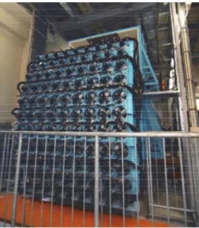
Figure 2.2 shows a multi-fan wind tunnel designed by, Japan, the jet device is composed of 9-row and 11-column array, i.e. a total of 99 fans, the test section size reaches 2.6 m * 1.8 m * 15.5 m. The rotational speed of each fan can be controlled independently by a computer for random fluctuation, a hot-wire anemometer can be used to measure the fluctuation velocity and its power spectrum downstream. After feedback and repeatedly and reversely adjusting for approximation, finally it can obtain a atmospheric boundary layer flow field that coincides with the characteristics of the target. This technology can simulate almost a wind velocity time series that is entirely consistent with the target wind field.
Fig 2.2 Multi-fan device in Miyazaki University
12
3. On the boundary layer formation of a small simple type wind tunnel
3.1 Wind tunnel structure
Figure 3.1 shows a diagram and a photograph of the wind tunnel used in this research.
The wind tunnel that was used is a single-circuit open-return wind tunnel and is composed of a fan, settling chamber, and test section. The length of the wind tunnel is 8.25 m, and its cross section is 0.8 m × 0.5 m. The length of the settling chamber is 3.6 m, and the length of the test section is 1.8 m.
Considering the fact that sand drift in the natural environment is most vigorous at heights below 0.3 m (Abulaiti and Kimura, 2011), the height of the wind tunnel was chosen to be 0.5 m in order to keep the wind tunnel small. The width of the wind tunnel was set to be less than 1 m in order to keep the wind tunnel small, assuming that a wind layer that is affected by friction is formed in an area 0.2 m from the inner side of both walls Yoshino et al. 1985 . The overall length of the wind tunnel and the lengths of the settling chamber and test section were chosen based on the outdoor wind tunnel of Tan and Zhang (2013) as a reference.
The exterior wall has a thickness of 0.8 cm and is made of acrylic. Acrylic was selected because it improves visibility of the condition of the sand drift as well as the process of the experiment. The thickness was chosen to be 0.8 cm because this thickness mitigates the degradation of the acrylic in our experience. The ceiling was designed to be removable so that it would be easy to set up the experiment.
The maximum output of the fan that was used in this experiment was 1.5 kW (Figure 3.2). The fan is equipped with an inverter (Figure 3.3), making it possible to change the wind velocity to according to the required wind velocity in the test section. The frequency can be adjusted from 0 Hz to 60 Hz, and the wind velocity of the wind created by the fan can be adjusted from 0 m/s to 12 m/s.
A hexagonal-type honeycomb (Figure 3.4) was placed at the exit of the fan. The purpose of the honeycomb is to straighten the flow of the turbulent air that is sent from
13
Fig 3.1 Schematic and actual photo of wind tunnel
14
Fig 3.2 Pictures of fan Fig 3.3 Pictures of inverter Fig 3.4 Pictures of honeycomb
15
the fan to flow in a constant direction. Increasing the length of the honeycomb results in more straightening of the air flow, but this also causes larger losses in the wind velocity.
Decreasing the diameter of the honeycomb cells also results in deceased turbulence intensity. The honeycomb that was used in this research was made of aluminum and had a thickness of 0.2 cm, length of 8 cm, and diameter of 2 cm, which were chosen based on the results in Mehta (1977).
16
3.2 Wind velocity measurement method
In this research, experiments were performed with the mainstream wind velocity maintained at a constant value of 8 m/s. The wind velocity was measured using a pitot tube (Figure 3.5) anemometer that was fixed to a stand. Moving observations of the wind velocity in the vertical direction and horizontal direction were taken on the upwind side of test section. The measurement axis for the vertical direction was chosen to be at the center of the upwind side of the test section. The measurement was performed in the height range of 0.4 cm - 50 cm (2 cm measurement interval). The measurement axis for the horizontal direction was chosen to be at the upwind side of the test section as well. The measurement was performed at a height of 4 cm and in the range of 0.4 cm - 78 cm from the wall (2 cm measurement interval). The measurement interval was chosen to be 2 cm based on the sensor specifications. The data was recorded at an interval of 1 second. 30 seconds of data were averaged and used for the analysis (Figure 3.6).
In order to measure the wind velocity profile in the vertical and horizontal directions for the case in which the ground is covered in sand, the measurement was taken with a wooden board with sand stuck onto it placed on the floor.
Fig 3.5 Picture of pitot tube
Fig 3.6 Picture taken from wind tunnel observation site
17
3.3 Boundary layer formation method and design of turbulence generator
3.3.1 Boundary layer formation method
Methods for reproducing boundary layers in wind tunnels can be categorized into two types: Methods in which the boundary layer is formed naturally, and methods in which the boundary layer is formed artificially. In methods in which the boundary layer is formed naturally, the boundary layer is formed naturally by walls of the same roughness. In order to form a boundary layer of thickness 0.5 - 1.0 m, a settling chamber of length 20 - 30 m is required. Considering the installation costs, such a settling chamber would be too long, making this method unrealistic.
In methods in which the boundary layer is formed artificially, the boundary layer is formed by placing turbulence generators in the settling chamber. In this experiment, we chose to design and deploy turbulence generators in order to adjust the boundary layer.
In this method, the turbulence generators receive the wind that is sent from the fan and artificially generate an exponential wind velocity profile along the height profile of the turbulence generators (Figure 3.7). In this case, a logarithmic distribution of the wind velocity is generated in the vertical direction, even when the settling chamber is short.
The turbulence generators that were used in this experiment include both spires, which are pyramid-shaped columns, and roughness blocks arranged along the floor.
Fig 3.7 Schematic diagram of the turbulence generator installation method
h
18
3.3.2 Design of spires and roughness blocks
The sizes of the spires and the roughness blocks must be determined based on the size of the wind tunnel. According to the research results presented in Irwin (1981), the height and width of the spires can be calculated using the following equations.
) 2 / 1 /(
39 .
1 a
h (4)
) 1 1 2 ( 5 .
0 a H
h b
(5) ))
2 / 1 )(
1 (
13 . 1 )
2 1 ( ( 2 ) 1
( 2 a a
a
a (6)
a a
H 1 (7)
Here, h represents the height of the spires (m), represents the thickness of the boundary layer (set to be 0.3 m in this research), b represents the width of the spires (m), a represents the exponent (set to the value for a sandy surface, or 0.1, in this research), and H represents the height of the wind tunnel (0.5 m). Based on the calculation results, the value of h is 0.23 m, and the value of b is 0.024 m (Figure 3.8a). In the research results presented in Irwin (1981), the spacing of the spires was set to be half of their height. However, in this research, the spacing of the spires was set to be 0.125 m, and 6 spires were installed (Figure 3.8b).
Figure 3.8 Schematic of spire (a) and pictures of installation (b)
In this experiment, the boundary layer was generated artificially in order to avoid using a long settling chamber that would have been required in order to form the
Front Side Base (a)
0.125m 1m
(b)
19
boundary layer naturally. However, if the length of the settling chamber is made short, it is difficult to make the profile of the wind velocity constant in the horizontal direction.
Therefore, in this research, cubic roughness blocks were placed downwind from the spires to adjust the wind velocity profile. The length of the sides of the roughness blocks can be calculated using the following equation (Irwin, 1981).
} ] 05 . 2 2 ) [(
1161 . 0 ) 3ln(
exp{2 12
Cf
D k
(8)
2
136 1 .
0 a
Cf a
(9)
Here, k represents the length of the sides of the roughness blocks (m), and D represents the spacing between the blocks (in this research, set to a value of 0.05 m). Based on the results of the calculation, the length of the sides of the roughness blocks k was set to 0.01 m.
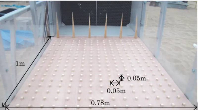
By using both spires and roughness blocks, it is possible to create a wind velocity profile in the vertical direction (or in other words, to generate a boundary layer) and it is possible to create a constant wind velocity profile in the horizontal direction. In this way, wind tunnels can be improved so that it is possible to perform sand drift experiments even with short settling chambers. An image of the installation of the spires and roughness blocks downwind is shown in Figure 3.9.
0.78m 1m
0.05m 0.05m
Fig 2.9 Schematic of installation of spire and roughness block
20
3.4 Results and discussion
Figure 3.10a shows the results of a measurement of the wind velocity in the vertical direction for the condition in which turbulence generators (in other words, spires and roughness blocks) were not used. The boundary layer thickness is determined from a logarithmic approximation using the observation points from the ground to the point where the wind velocity ceases to increase with height. As a result, the thickness of the boundary layer was determined to be 14 cm, which is fairly thin. Examining the wind velocity profile in the horizontal direction (Figure 3.10b) reveals that the wind velocity in the area that is between 20 cm and 60 cm is not affected by the wall. In addition, the standard deviation of the wind velocity profile in the horizontal direction (between 20 cm and 60 cm) is 0.12 m/s, which indicates that the turbulence was relatively large.
Next, Figure 3.11a shows the results of the measurement of the vertical profile of the wind velocity for the condition in which only the spires were used. The thickness of the boundary layer increased by 4 cm, which is a small amount (18 cm). The deviation from the line showing the logarithm approximation decreased greatly compared to the case in which spires were not used. In the horizontal direction (Figure 3.11b), using the spires caused the standard deviation of the wind velocity profile in the horizontal direction to increase (0.17 m/s). These results imply that using spires alone enables the wind velocity profile in the vertical direction to be adjusted somewhat, but also disturbs the wind velocity profile in the horizontal direction.
Next, Figure 3.12a shows the results of the measurement of the vertical profile of the wind velocity for the condition in which both the spires and the roughness blocks were used. The spacing of the roughness blocks in Figure 3 was 5 cm. This value is the initial value for the spacing, but it is also possible to adjust this value based on the results. As a result, the thickness of the boundary layer increased by 20 cm (38 cm). By using the roughness blocks, it is possible to generate a boundary layer that can withstand the sand drift experiments. In the horizontal direction, the standard deviation of the wind velocity profile in the horizontal direction was not very different from the case in which only spires were used (0.19 m/s) (Figure 3.12b). However, the wind velocity profile differs from the profile shown in Figure 5b in that the wind velocity profile in the horizontal direction has been made uniform at intervals of approximately 5 cm due to the effect of setting the spacing between the blocks to 5 cm. Comparing the roughness lengths
21
Fig 3.10 Wind velocity distribution in the vertical direction when only the honeycomb is installed (a) and wind speed distribution in the horizontal direction (b)
Fig 3.11 Distribution of wind velocity in the vertical direction when spire is installed (a) and wind speed distribution in the horizontal direction (b)
Fig 3.12 Distribution of wind velocity in the vertical direction when spire and roughness block are used together (a) and wind speed distribution in the horizontal direction (b)
(a)
0.0001 0.001 0.01 0.1 1 10 100
0 2 4 6 8 10
Wind speed(m/s)
(a)
0.0001 0.001 0.01 0.1 1 10 100
0 2 4 6 8 10
Wind speed(m/s) Wind Speed(m/s)
3 4 5 6 7 8 9
0 20 40 0 6 80 100
(b)
(a)
0.0001 0.001 0.01 0.1 1 10 100
0 2 4 6 8 10
Wind speed(m/s) Wind speed(m/s)
3 4 5 6 7 8 9
0 20 40 0 6 80 100
(b)
Wind speed(m/s)
3 4 5 6 7 8 9
0 20 40 0 6 80 100
(b)
22
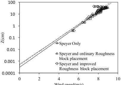
between the case in which roughness blocks were used and the case in which roughness blocks were not used (Figure 3.13), it can be seen that the roughness length (y-intercept) at the downwind side of the test section was slightly larger when roughness blocks were used, although the difference was not very large. Considering the fact that the roughness length of flat bare land in the natural environment is 1 order of magnitude larger (0.01 cm: Kondo, 1994), this difference is small.
Since the change in the wind velocity profile in the horizontal direction is still large, we investigated and proposed a method for improving the arrangement of the roughness blocks. This method involves combining spires with roughness blocks arranged in two different arrangement densities in order to adjust the wind velocity profile of the
0.0001 0.001 0.01 0.1 1 10 100
0 2 4 6 8 10
Wind speed(m/s) Speyer Only
Speyer and ordinary Roughness block placement
Speyer and improved Roughness block placement
5cm
5cm
2.25cm 90cm
30cm
Fig 3.13 Comparison of wind speed distribution and roughness length in the vertical direction with and without roughness block
Fig 3.14 Appearance of roughness block devised newly
23 (a)
0.0001 0.001 0.01 0.1 1 10 100
0 2 4 6 8 10
Wind speed(m/s) Wind speed(m/s)
3 4 5 6 7 8 9
0 20 40 0 6 80 100
(b)
boundary layer in the vertical direction while adjusting the wind velocity profile in the horizontal direction with the roughness blocks.
The idea proposed for the roughness block arrangement densities is shown in Figure 3.14. In the arrangement density proposed in this research (Figure 3.14), the arrangement density in the length direction was increased in order to make the sizes of the turbulence vortices smaller and to make the wind velocity profile in the horizontal
direction approximately uniform. The results show that although the thickness of the boundary layer did not change (38 cm) (Figure 3.15a), the standard deviation of the horizontal wind velocity profile became 0.08 m/s (Figure 3.15b), which implies that the horizontal wind velocity profile was made approximately uniform. It is anticipated that fine-tuning the spacing of the roughness blocks will result in further improvement of the horizontal wind velocity profile. However, since the accuracy of the profile that was obtained in this experiment was already sufficient (much smaller than the measurement precision of the pitot tube (0.25 m/s)), no further investigation was conducted as part of this research.
Fig 3.15 Wind velocity distribution in the vertical direction when roughness block arrangement density is changed (a) and Wind speed distribution in the horizontal direction (b)
24
3.5 Conclusion
In this research, a method for generating a boundary layer in a small-scale simple wind tunnel using both spires and roughness blocks was proposed. In addition, a method for adjusting the wind velocity profile in the horizontal direction to make it uniform as well as forming a boundary layer was also proposed. The method resulted in a boundary layer with a thickness of 38 cm in a settling distance of 3.6 m. In addition, it was possible to make the wind velocity profile approximately uniform in the horizontal direction by adjusting the arrangement of the roughness blocks. By using spires and roughness blocks together in this way, it is possible to design low-cost small-scale simple wind tunnels with short settling distances. In this research, the dimensions of the wind tunnel were designed beforehand based on estimates for the thickness of the boundary layer required for measurements. The thickness of the boundary layer was further adjusted after completion of the wind tunnel.
In the future, we plan to use this wind tunnel for environmental experiments such as studying wind ripples, sand saltation, mechanisms of yellow dust generation, and countermeasures for yellow dust.
25
4 A method to make a boundary layer with roughness length
4.1 Introduction
In order to observe sand drift phenomena using wind tunnels, it is important to ensure that experiments are not affected by measurement conditions such as irregular changes in the wind direction and wind velocity (Arien, 1978). Furthermore, it is important to be able to recreate conditions that are similar to the conditions of the natural environment while being able to freely set the experiment parameters. In particular, two conditions that are necessary for wind tunnel experiments include the boundary layer and roughness length, which affect the vertical distribution of the amount of sand drift, and a stable wind velocity profile in the test section.
Liu and Kimura (2016) used devices for controlling the turbulence of the wind spires and roughness blocks) and proposed a method for achieving a flow that has properties that are similar to the atmospheric boundary layer within relatively short settling distances. As a result, the researchers were able to obtain a boundary layer of a thickness of 38 cm within a short settling distance of 3.6 m. Furthermore, by adjusting the arrangement of the roughness blocks, the researchers were able to make the wind velocity in the test section approximately uniform in the horizontal direction. However, the roughness length in the test section was 0.001 cm, which is small. This value is one order of magnitude smaller than the roughness length of flat bare land in the natural environment (for example, 0.01 cm; Kondo, 1994).
In order to use spires and roughness blocks to achieve this roughness length, it is necessary to adjust the resistance to the wind in the settling chamber. In general, the roughness length can be adjusted by changing the sizes of the roughness blocks, the horizontal and vertical spacing of the roughness blocks, and the number of columns
Sill,1988 Yi and Tian,2013 . However, previous research does not provide any methods or procedures for simultaneously achieving roughness lengths that are close to the value found in a natural environment, wind velocity profiles that are constant in the
26
horizontal direction, and stable wind velocities within the test chamber while maintaining the thickness of the boundary layer at a stable value. The goal of this research is to propose a method/procedure for satisfying these conditions simultaneously using turbulence control devices (spires and roughness blocks) based on the simple small-scale wind tunnel described in Liu and Kimura (2016).
27
4.2 Overview of simple wind turbine and wind velocity measurement method
The wind tunnel used in this experiment is a single-circuit open-return wind tunnel and is capable of generating a boundary layer (Liu and Kimura, 2016). The wind sent from the fan (maximum output 1.5 kW) passes through the honeycomb that has been installed to straighten the flow. After a turbulent flow is formed in the settling chamber of nominal dimensions 3.6 m × 0.8 m × 0.5 m, a boundary layer with a thickness of 0.38 m can be formed in the test section of dimensions 1.8 m × 0.8 m × 0.5 m. A diagram and a photograph of the wind tunnel are shown in Figure 3.1. The fan is equipped with an inverter, so the wind velocity produced by the fan can be freely set according to the requirements of the measurement (0 m/s 12 m/s).
For measuring the wind velocity, the mainstream wind velocity was set to a constant value of 8 m/s, identical to the method in Liu and Kimura (2016). Moving observations of the wind velocity in the vertical direction and horizontal direction were taken on the upwind side of test section using a pitot tube flow velocity/flow rate micro differential pressure gauge (MK Scientific, Inc.: DT-8920) that was fixed to a stand. The measurement axes in the vertical direction and the horizontal direction were aligned along the height (0.5 m) and width (0.78 m) of the wind tunnel. Measurements were taken at measurement intervals of 0.02 m. The measurement axis for the vertical direction was chosen to be at the center of the upwind side of the test section. The wind velocity profile in the horizontal direction was measured at a height of 4 cm from the floor of the test section. The data was recorded at an interval of 1 second. 1 minute of data was averaged and used for the analysis. In order to measure the wind velocity profile in the vertical and horizontal directions for the case in which the ground is covered in sand, the measurement was taken with a wooden board with sand stuck onto it (fixed to the surface of the wooden board with adhesive) placed on the floor from the settling chamber to the test section.
28
4.3 Proposal for method which simultaneously achieves roughness length, boundary layer thickness, uniform wind velocity profile in the horizontal direction, and test section with stable wind velocity
4.3.1 Roughness length adjustment method
According to the results presented by Sill (1988), there are two methods for increasing the roughness length using only roughness blocks: Increasing the number of vertical columns without changing the size of the roughness blocks and the spacings of the roughness blocks in the horizontal and vertical directions (horizontal and vertical lengths with respect to the wind direction on the surface on which the roughness blocks are laid: Refer to Figure 4.2), and changing the size of the roughness blocks and the spacings of the roughness blocks in the horizontal and vertical directions without changing the number of columns. In method , it is possible to adjust the roughness length to a certain extent just by increasing the number of columns. However, increasing the number of columns makes it necessary to increase the length of the settling chamber (Yi and Tian, 2013). Therefore, this method is not a realistic option for designing a wind tunnel with a short settling chamber, which is the goal of this research.
In method , the effect of the roughness blocks extends to an area that is only 5 times the height of the roughness blocks (Sill, 1988). In other words, since the roughness blocks mainly adjust the lower layers of the boundary layer, in order to adjust the upper layers of the boundary layer, it is necessary to set the sizes of the roughness blocks to be complex. For example, using roughness blocks of different heights at the same time enables the vertical profile of the wind velocity to be adjusted. However, one shortcoming of this method is that it requires a large amount of trial and error and much time.
Liu and Kimura (2016) proposed a method for generating boundary layers that are required for performing sand drift experiments using spires and roughness blocks together. The functions of the spires and roughness blocks are shown in Table 4.1. The results show that the spires and roughness blocks provide resistance to the wind sent from the fan, and are helpful in generating boundary layers that are relatively thick.
However, the wind velocity profile in the vertical direction is affected by the spires
29
more than the roughness blocks (Table 4.1). Therefore, we focused on the wind-receiving area of the spire, and hypothesized that minute changes in the wind-receiving area can have an effect on the wind velocity profile in the vertical direction and on the upper layers of the boundary layer in particular. In this research, we propose a method for generating boundary layers that accompany roughness lengths that are similar to those found in natural environments by adjusting the shape of the spires.
Table 4.1 Role of spiers and roughness blocks
Role of speyer Role of roughness block
Adjustment of boundary layer thickness
(Particularly in the upper part)
Adjustment of boundary layer thickness (Particularly in the lower part)
Vertical wind speed distribution Fine adjustment of wind speed distribution in the vertical direction
Horizontal wind speed equality
30
4.3.2 Adjustment of spire shape
The height (0.23 m) and width (bottom side of the triangle of the bottom face: 0.024 m) of the spire were chosen based on the research presented by Liu and Kimura (2016) and Irwin (1981). In order to increase the wind-receiving area of the spires without changing their height or width, we considered increasing the width of the top end of the spires. This change caused the shape of the wind receiving face of the spires to change from a triangle shape to a trapezoidal shape (hereafter, we refer to these spires as trapezoidal spires). The width of the top end of the trapezoidal spires was chosen to be 0.003 m, based on the results presented by Ham and Bogusz (1998) (Figure 4.1a).
Similar to Liu and Kimura (2016), 6 spires were lined up horizontally with a spacing of 0.125 m (Figure 4.1b). In order to increase the resistance to the wind, the material used for the spires was changed from wood to acrylic board with a thickness of 0.05 m. The roughness blocks (height 0.1 m, width 0.09 m) were arranged with a spacing of 5 cm in an area of length 0.55 m and width 0.6 m, similar to the arrangement used by Liu and Kimura (2016). Furthermore, additional roughness blocks were paced downwind with an increased density with a spacing of 2.5 cm in an area of length 0.25 m and width 0.5 m (indicated by numbers in Figure 4.2).
In this research, we hypothesized that trapezoidal spires and roughness blocks can be used together to generate boundary layers that are relatively thick and have roughness lengths that are similar to those of the natural environment while maintaining the uniformity of the wind velocity profile in the horizontal direction and maintaining the stability of the wind direction and wind velocity in the test section. Figure 4.2 shows a photo of how the trapezoidal spires and roughness blocks are installed.
31
Fig 4.2 Overview of installation of trapezoid spears and roughness blocks in the rectification field
Fig 4.1 Trapezoid spire specification (a) and installation overview (b) Front Side Bottom
(a) (b)
0.7m
0.125m 0.8m
0.25m
32
4.4 Results and discussion
4.4.1 Generation of a boundary layer with roughness length that is similar to that of the natural environment
Figure 4.3a shows the results of a measurement of the wind velocity profile (in the vertical direction) for the condition in which both trapezoidal spires and roughness blocks were used. The thickness of the boundary layer was 0.34 m. This result is almost identical to the result of Liu and Kimura (2016). However, the roughness length increased by one order of magnitude and became approximately 0.01 cm. Making the
Wind speed(m/s)
3 4 5 6 7 8
0 20 40 60 80 100
0.001 0.01 0.1 1 10 100
0 2 4 6 8 10 21
Z (cm)
Wind speed (m/s)
Figure 4.3 Vertical wind speed distribution (a) and horizontal wind speed distribution (b) when trapezoid spear and roughness block are used in
33
wind-receiving face of the spires trapezoidal in shape enabled us to generate a boundary layer that was relatively thick and increase the roughness length at the same time.
However, the variation in the wind velocity profile in the horizontal direction (taken at a height of 4 cm and width of 20 cm to 60 cm away from the wall) was large. The standard deviation of the difference of the wind velocity was 0.15 m/s (Figure 4.3b).
Compared to the results presented by Liu and Kimura (2016), the variation increased by a factor of 2.
Therefore, in order to make the wind velocity profile in the horizontal direction more uniform, we tried changing the arrangement of the roughness blocks downwind. Since changing the arrangement of the blocks would require a large amount of time for measurement, wind velocity data was taken only in the range from 20 cm to 60 cm away from the wall for measuring the wind velocity profile in the horizontal direction.
The difference in the wind velocity profiles in the horizontal direction caused by the difference in the arrangement of the blocks is shown in Figure 4.4. In case a, 20 roughness blocks were added with a spacing of 2.5 cm over an area of vertical width 0.1 m and horizontal width 0.5 m. As a result, the standard deviation of the difference in the wind velocity in the horizontal direction became 0.33 m/s. In case b, 40 roughness blocks were added with a spacing of 2.5 cm over an area of vertical width 0.2 m and horizontal width 0.2 m on the side of the left wall, and over an area of vertical width 0.2 m and horizontal width 0.3 on the side of the right wall (the resulting standard deviation was 0.27 m/s). In case c, 46 roughness blocks were added with a spacing of 2.5 cm over an area of vertical width 0.2 m and horizontal width 0.6 m (the resulting standard deviation was 0.28 m/s). In case d, 102 roughness blocks were added with a spacing of 2.5 cm over an area of vertical width 0.35 m and horizontal width 0.6 m (the resulting standard deviation was 0.26 m/s).
Examining the results shown in Figure 4.4 shows that the wind velocity profiles in cases a, c, and d have only a narrow range in which the wind velocity is uniform. On the other hand, although the value of the standard deviation of the difference in wind velocity shown in case b is no different (compared to the other cases), the range in which the wind velocity is uniform is large. However, the value of the standard deviation of the difference of the wind velocity did not improve compared to its value
34
Fig 4.4 Relationship between roughness block arrangement method and horizontal wind speed distribution Wide(cm)
Wide (cm ) Wid
e(cm )
Wide (cm)
35
Fig 4.5 New arrangement of trapezoid spire
before the arrangement of the roughness blocks was changed (0.15 m/s). In other words, these results indicate that changing the arrangement of the roughness blocks does not have a large impact on the uniformity of the wind velocity profile in the horizontal direction.
Therefore, we shifted focus to the spires again. We hypothesized that it is possible to decrease the turbulence intensity without affecting the shape of the boundary layer, or in other words to make the wind velocity profile in the horizontal direction become uniform, by decreasing the area of the wind tunnel cross-section that captures the wind without changing the slope angle of the spires (angle between the diagonal side and bottom side). In order to validate this hypothesis, we decreased the number of spires from 6 to 5 without changing the spacing (Figure 4.5). The roughness blocks were arranged in the same way as was done by Liu and Kimura (2016). The wind velocity profile in the vertical direction is shown in Figure 4.6a. The thickness of the boundary layer was 38 cm. Although the standard deviation of the difference of the wind velocity in the horizontal direction decreased to 0.09 m/s (Figure 4.6b), the range in which the wind velocity is approximately constant is biased to one side (26 cm - 68 cm), and the
36
wind velocity still has large variation especially in the range from 16 cm - 20 cm. We tried to identify the cause of the variation in the range from 16 cm - 20 cm. In this research, we designed the trapezoidal spires to have a top end width of 0.003 m.
However, the acrylic boards were thick (0.005 m) and difficult to machine with high precision, so we were unable to make their widths strictly uniform (Figure 4.6). In other words, we believe that the reason for the variation in the wind velocity profile in the horizontal direction is the fact that the slope angles of the spires are not uniform.
Wind Speed(m/s)
4.0 4.5 5.0 5.5 6.0 6.5 7.0 7.5 8.0
0 20 40 60 80 100
0.001 0.01 0.1 1 10 100
0 2 4 6 8 10
Z (cm)
Wind speed (m/s)
Fig 4.6 Vertical vertical wind speed distribution (a) and horizontal wind speed distribution (b) when newly devised speyer is placed.
37
Therefore, in order to make the widths of the top ends uniform, we changed the thickness of the acrylic boards to 0.003 m, and redesigned the widths of the top ends to be 0.005 m. Since the 0.003 m acrylic boards are thin, there is a chance that vibrations will occur during experiments with high winds. In order to overcome this issue, we installed triangular struts of height 0.15 m to the spires (Figure 4.7). 5 spires were lined up horizontally at a spacing of 0.125 m (Figure 4.8). The roughness blocks were arranged in the same way as was done by Liu and Kimura (2017). As a result, the boundary layer thickness was unchanged at 38 cm. However, the standard deviation of the difference of the wind velocity in the horizontal direction became 0.1 m/s, which is smaller, and the range in which the wind velocity was uniform was not biased (Figure 4.9). In the end, we were able to generate a boundary layer with a roughness length that is close to that found in the natural environment while simultaneously creating a wind velocity profile that is uniform in the horizontal direction without changing the arrangement or density of the roughness blocks and by adjusting only the spires.
Fig 4.7 New trapezoid spire specification
Front Side Bottom
38
Fig 4.8 Pictures of the turbulence generator installation method
Fig 4.9 Vertical wind speed distribution (a) and horizontal wind speed distribution (b) when new trapezoid spire and roughness block are used together.
0.001 0.01 0.1 1 10 100
0 2 4 6 8 10
Wind speed(m/s)
WindSpeed(m/s)
3 4 5 6 7 8
0 20 40 60 80 100