JAIST Repository: Study on tensor calculus and CP-decomposition

(1)

Japan Advanced Institute of Science and Technology

JAIST Repository

https://dspace.jaist.ac.jp/

Title Study on tensor calculus and CP-decomposition Author(s) Nguyen, Linh

Citation

Issue Date 2015-03

Type Thesis or Dissertation Text version author

URL http://hdl.handle.net/10119/12686 Rights

(2)

Master Dissertation

Study on tensor calculus and CP-decomposition

NGUYEN VU LINH

Major in Knowledge Science

School of Knowledge Science

Japan Advanced Institute of Science and Technology

(3)

Master Dissertation

Study on tensor calculus and CP-decomposition

By Nguyen Vu Linh (1350016)

Supervisor: Professor Ho Tu Bao

Major in Knowledge Science

School of Knowledge Science

Japan Advanced Institute of Science and Technology

Written under the direction of

Professor Ho Tu Bao

and approved by

Associate Professor Dam Hieu Chi

Associate Professor Huynh Van Nam

Professor Tsutomu Fujinami

February 2015 (Submitted)

(4)

(5)

Abstract

Study on tensor calculus and CP-decomposition

Nguyen Vu Linh (1350016)

School of Knowledge Science,

Japan Advanced Institute of Science and Technology March 2015

Keywords: Tensor, CP-decomposition, Multi-way array, Temporal link prediction, Spectral clustering.

Tensor have been widely studied in mathematics and physics for along time and increas-ingly applied in many areas of data mining. There are two ways to think about tensors: tensors are representations of multilinear maps; tensors are elements of a tensor product of two or more vector spaces. For our purpose, “a Nth_{-order tensor” is defined as “an element}

of tensor product of N real vector spaces V1, V2, . . . , VN, denoted by V1⊗ V2⊗ . . . ⊗ VN.

When fixing the bases of V1, V2 and VN, a tensor can be represented by a N ”-way array

in the vector space Rd1×d2×...×dN _{and elements in V}

n can be represented as vectors in Rdn,

where dn is the dimension of Vn.

The equivalence between two vector space Rd1 _{⊗ R}d2 _{⊗ . . . ⊗ R}dN _{and R}d1×d2×...×dN allows us to not distinguish these two spaces. Such equivalence provides great advan-tages for data mining applications because N -way array may provide nature and compact representation for numerous complex kinds of data that the integrated result of several inter-related variables or they are combinations of underlying latent components or fac-tors. Furthermore, when considering N -way array as element of Rd1×d2×...×dN_{, powerful} results related to tensor can be employed to construct tensor based methods to solve challenging problems. Especially, when working with challenging problems for big data related to capture, manage, search, visualize, cluster, classify, assimilate, merge, and pro-cess the data within a tolerable elapsed time. When working on tensor data, the large required storage memory and the inter-relation between variables often make the prob-lems become more complicated. Many tensor-based models known as multiway models

(6)

have been constructed to deal with those challenges by exploring the meaningful hidden structure and to finding low-rank representation of data. Also, each kind of model have its own advantages and disadvantages which should be carefully considered based on the application context. For example, using CP-decomposition may lead to losing important data structure while Tucker decomposition may be problematic in high-dimensions with many irrelevant features.

One interesting tensor-based method is temporal link prediction method based on CP-decomposition constructed to do temporal link prediction task on bipartite networks whose links evolve over time and node set consists vertices of two types such that only vertices of diffent types can be linked. Such problem is important and has been stud-ied in many researches because prediction is crucial tasks in real applications and bi-partite networks can be used to represent various kinds of structures, dynamics, and interaction patterns found in social activities. Temporal link prediction method based on CP-decomposition have shown advantages comparing with others, such as its power in exploring the structure of data, requiring less memory and giving outperformed experi-mental results. Also, tensor based-methods can predict the links for times (T + 1)th, . . . , (T + L)th _{while other models are limited to temporal prediction for a single time step.}

Motivating by these advantages, we extend tensor-based method on bipartite networks to do temporal link prediction problem on specific class of bipartite networks in which new verticies of one type may join networks at concerning time and may link to other vertices in the next time point. The key ideas of the proposed methods are to employ CP-decomposition to decompose weight data into factors of three separated kinds, each fluctuates independently from others and collect additional information of vertices of open type and learn a function to predict values of open type vertex factors from the additional information and use to predict values of those factors corresponding to new vertices.

Clustering plays an outstanding role in numerous data mining applications such as scien-tific data exploration, information retrieval and text mining, spatial database applications, Web analysis, CRM, marketing, medical diagnostics, computational biology, and many others. Intuitively, clustering aims to identify groups of “similar behavior” data considered as a first impression on data when dealing with the empirical data. Since tensor data have became popular in data mining, we focus on constructing a versatile clustering for tensor data. Considering clustering methods based on vector space model, spectral clustering have several attractive advantage such that it is versatile, easy to implement, often pro-vide better performance comparing with traditional methods like K-mean. Furthermore, spectral clustering is easy to extend for tensor data since it work with only requirement about similarity while other methods often require more additional information. To han-dling the clustering task on tensor data, we construct a CP-decomposition based spectral clustering by constructing appropriate similarities and employing CP-decomposition to exploring the hidden structure of data and reducing the storage memory. The empirical results provide the evidence to conclude that the proposed models can give the acceptable accuracy and CP-decomposition may help to reduce the storage memory and improve the clustering accuracy by exploring the hidden structure of data.

(7)

achievements and provide suggestions to and make plan to complete these objective as future works. For temporal link prediction problem, we plan to implement the method and evaluate using empirical results and extend method to do more general problem when vertices of two type join the concerning networks at the same time. Considering the clustering problem, we plan to construct several similarity measures and extend the available vector space model based multi-view spectral clustering for tensor data. We also give opportunity and suggestions to construct a tensor space model based clustering method which tensor data is transformed in to vector space data and spectral clustering methods are applied on the transformed data in order to cluster the data.

(8)

Acknowledgments

I would like to express my deep gratitude to my master thesis advisor Professor Ho Tu Bao of Japan Advanced Institute of Science and Technology. He did introduce me to the research field of machine learning and data mining and spend much time instructing me how to do research. Becoming his student is one of biggest chances for me.

I would like to show my gratitude to the committee members, Professor Dam Hieu Chi, Professor Katsuhiro Umemoto, Professor Huynh Van Nam and Professor Tsutomu Fujinami of Japan Advanced Institute of Science and Technology, for their insightful and constructive comments that helped to improve the presentation of this thesis.

I would like to thank my second supervisor Professor Yukio Hayashi and my supervisor for minor research Professor Mitsuru Ikeda of Japan Advanced of Science and Technology for their suggestions and continuous encouragements.

I am grateful to Japan Advanced Institute of Science and Technology for providing me finance support and a good environment to study.

I would also like to thank all members of Ho Laboratory who are great friends and helpful to color my life.

Finally, I owe more than thanks to my family for their loves and encouragement during the duration of Master’s course.

Nguyen Vu Linh JAIST, Japan February, 2015

(9)

List of Figures

1.1 List of popular multi-way models (tensor based models) [3]. . . 3

2.1 Fibers of a 3rd_{-order tensor [38]. . . .} ₉

2.2 Slices of a 3rd_{-order tensor [38]. . . .} ₁₀

2.3 The frontal slices of tensor [38]. . . 10

2.4 The three mode-n of tensor [38]. . . 10

2.5 Commutative diagram [21]. . . 13

2.6 CP decomposition of a third order tensor [38]. . . 15

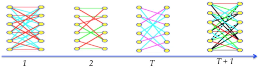
3.1 An example of bipartite network that evolve over time. . . 19

3.2 An example of open bipartite network that evolve over time. . . 19

3.3 Illustration of temporal link prediction method proposed in [2, 26]. . . 20

4.1 Image of a Blue Crab. . . 33

4.2 The point-pairs result [57]. . . 35

4.3 Experimental result on 4 datasets. . . 36

4.4 Comparison between single view (left) and multi-view (right) spectral clus-tering [48]. . . 37

4.5 A tensor space model based clustering method. . . 39

(11)

List of Tables

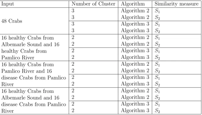
2.1 List of important notations. . . 9 2.2 Models in PARAFAC family [3]. . . 16 4.1 Description of experiments. . . 34 4.2 Comparing results of Algorithm 2 (S2) and highest result of Algorithm 4. . 40

(12)

Chapter 1 Introduction

The first part of this chapter provides an overview of tensor calculus and its role in data mining. In the second part, the research problems and objectives are presented. Finally, the content of this thesis is given in the third part.

1.1 Tensor calculus and its role in data mining

1.1.1 Tensor calculus

Tensor have been widely studied in mathematics and physics for along time and increas-ingly applied in many areas of data mining. There are two ways to think about tensors: tensors are representations of multilinear maps; tensors are elements of a tensor product of two or more vector spaces [21,45,60]. In this thesis, we use the definition of tensor that “a Nth_{-order tensor is an element of tensor product of N vector spaces V}

1, V2, . . . , VN,

denoted by V1 ⊗ V2 ⊗ . . . ⊗ VN, which is represented by a N ”-way array or element of

vector spaces Rd1×d2×...×dN _{when the bases of V}

1, V2 and VN are fixed.

Tensor and tensor product of vector spaces are difficult objects in algebra. Those objects have been studied for along time in algebra areas like tensor algebra and multilinear algebra [11, 19, 24, 30, 49, 55, 66, 70]. To understand the properties of those objects, deep understanding about vector space, relation between vector space and other algebra objects including multi-linear function, quotient spaces, etc are required. There are some readable documents about tensor, tensor product of vector spaces and related results in general case, for example [49, 60].

In this thesis, we consider one specific case of 3rd_{-order tensor as element of tensor}

product of 3 Euclidean vector spaces RI, RJ and RT, denoted by RI ⊗ RJ

⊗ RT_{, which}

is not so complicated but have been widely applied in multi-way data analysis [3, 19, 38]. Also the definition of tensor product of vector spaces is not presented here because it is complicated and we only work on the vector space constructed on the set of 3 real way arrays, denoted by RI×J ×T_{. Vector space R}I_{⊗ R}J_{⊗ R}T_{, and the relation between R}I_{, R}J

and RT _{have been well studied in algebra. Furthermore, as point out in [21], the structure}

of two vector spaces RI⊗ RJ

⊗ RT

(13)

RI⊗ RJ ⊗ RT can be easily proved on RI×J ×T.

1.1.2 Tensor-based models in data mining

Data representation has been considered as one of the most important problem in machine learning and data mining [12, 33]. Many applications are based on vector space model in which data is represented as vectors x ∈ RI_{. In vector space model, the features are}

implicitly assumed to be independent [12]. Vector space model have been used to construct many models, for example, classification, clustering [54], support vector machine, etc. There are numerous readable documents about vector space based models [33, 54, 64].

However, in many situations, there are reasons to consider data as tensors. For example, multi-channel electroencephalogram (EEG) data are commonly represented by an I × T matrix which represents recorded signals of I electrodes at T times. In order to discover hidden brain dynamics, often frequency content of the signals like signal power at J particular frequencies, also needs to be considered. Then, EEG data can be arranged as an 3-way dataset of size I × J × T [50]. Similarly, a 3-way tensor X of size I × J × T can be used to represent the publication information of I authors on J conferences over T years, where element xijt is 1 if authors i have publication on conference j at year t

and is 0 if otherwise [2, 26].

Generally, tensors can be used to represent several complex kinds of data that the integrated result of several inter-related variables or they are combinations of underlying latent components or factors [18]. For instances, 3-order tensors can be used to represent multi-view data [48], time series data [2, 26], etc. When tensors are used to represent data, we work on tensor space model instead of vector space model [13, 34, 50, 56, 59, 69]. Note that, when working with vector space models RI_{, a I × J matrix is often used}

to represent a dataset consists of J samples. Further more, as matrix have been well studied in linear algebra, many interesting results can be employed when handling data. For example, one may apply matrix factorization models to explore the structure of data or find low-rank representation. Some popular matrix factorization methods are LU, QR, SVD, etc. The situation is similar when working with tensor space models. When tensors are used to represent data, tensor based methods allows us to discover meaningful hidden structures of complex data and to perform generalizations by capturing multi-linear and multi-aspect relationships [17].

Tensors and tensor based methods have recently became a promising direction in many areas, especially in data mining because it may provide a natural representation for Big Data which consists of multidimensional, multi-modal datasets which are so huge, complex and cannot be easily stored or processed by using standard computers. Many challenging problems for big data are related to capture, manage, search, visualize, cluster, classify, assimilate, merge, and process the data within a tolerable elapsed time. Such problems can be solved by employing tensor decomposition models (or multi-way models), which allow us to discover meaningful hidden structures of complex data and provide compact representation via suitable low-rank approximations [3, 17, 18, 38].

There many tensor decomposition models and each kind of model have its own ad-vantages and disadad-vantages when comparing with others. For example, ones may lose

(14)

important structure in the data when using CP-decomposition while Tucker decomposi-tion may be problematic in high-dimensions with many irrelevant features [6, 7]. Some popular multi-way models (tensor based models) are listed in Figure 1.1.

Figure 1.1: List of popular multi-way models (tensor based models) [3].

1.2 Problem formulating and objectives

1.2.1 Constructing a temporal link prediction method on open

bipartite networks evolve over time

Temporal link prediction is a common problem for data which is assumed to have the underlying periodic structure. Formally, temporal link prediction is the problem of pre-dicting the links at time (T + 1)th _{given link data for times 1 through T}th _{[2, 26]. In}

other words, we consider the problem of predicting the change or apparition of new links in time-evolving networks. Temporal link prediction is different from simply predicting future links without considering the network evolution history because it exploits the past history of link evolution provided by the state of the network at successive time slices [27]. In many applications dealing with temporal link prediction, data can be represented in form of bipartite networks with two set of vertices and only vertices of different types can be connected by links [2, 26, 43]. Considering bipartite networks that evolve over time, two sets of vertices are fixed and only the link between different kind of vertices change. Bipartite networks can be used to represent various kinds of structures, dynamics, and interaction patterns found in social activities [8, 22, 52, 53, 67]. For example, bipartite network is used to represent the network consists of I authors and J conferences where each link represents the possibility that an author publishes on a conference and temporal link prediction is used to predict which authors will publish at which conferences in year (T + 1)th _{given the publication data for the T previous years [2, 26]; I users/groups of}

(15)

a bipartite network [67]; Another example is the bipartite network consists of I patient groups and J drugs with the links represent the adverse effect of drugs.

Many temporal link prediction methods are based on matrix calculus which collapse the data into a single matrix by summing (with and without weights) the matrices correspond-ing to the time slices and uscorrespond-ing the result matrix to predict the network links in the next time points. Such methods have been successfully applied in several applications. For ex-ample, data about co-authorship networks extracted from arXiv [3, 26, 27], etc. However, the matrix-based methods are limited to temporal prediction for a single time step while in many applications, we wish to predict the links for a period of time starting at (T + 1)th

or in other words, for times (T + 1)th, . . . , (T + L)th. Recently, tensor-based methods were proposed which can be used in solving both single step and periodic temporal link prediction problems [3, 26, 27, 61]. In other words, tensor-based methods can be used to extend the application context of matrix based methods. In tensor-based methods, tensor decomposition namely CP-decomposition (CANDECOMP/PARAFAC) is employed with several purposes such as to explore the natural three-dimensional structure, reduce tensor dimensionality or to retrieve latent trends [3, 61].

When using bipartite networks to represent data, we may face some special bipartite networks with common situation that new vertices may join network at time Tth _{and may}

link to other vertices at time (T + 1)th. For example, when a bipartite network is used to represent data in recommendation system, new users/groups of user appear and may interest or use service of providers in next time points; also in drug side effect example, new drugs are launched and may have adverse effect on patient groups in the future; etc. For simplicity, let call such networks by open bipartite networks to distinguish from networks without new added vertices.

Several temporal link prediction methods have been proposed for bipartite networks [2, 23, 26] but in our knowledge, no temporal link prediction method have been proposed to deal with problem on open bipartite networks. In our point of view, temporal link prediction is challenging because it is difficult to learn how new vertices will link to other vertices and how it effects links among previous vertices at time (T + 1)th. Our objective is to extend temporal link prediction method using CP-decomposition in [2,26] to address temporal link prediction in open bipartite networks in which new vertices of type-1 may join networks at time Tth.

1.2.2 Constructing a versatile clustering method for tensor data

Clustering is an important subject of active research areas in several fields such as statis-tics, pattern recognition, machine learning and data mining which aims to identify groups of “similar behavior” data. In machine learning and data mining, clusters correspond to hidden patterns and is often referred as a first impression on data when dealing with the empirical data. Clustering plays an outstanding role in numerous data mining applications such as scientific data exploration, information retrieval and text mining, spatial database applications, Web analysis, CRM, marketing, medical diagnostics, computational biology, [9, 44, 57, 64], and many others.

(16)

Many clustering algorithms have been proposed and successfully applied to real-life data mining problems. A list of popular clustering methods and algorithms is given bellow [9].

1. Hierarchical methods: Agglomerative algorithms, divisive algorithms.

2. Partitioning methods: Relocation algorithm, probabilistic clustering, K-medoids methods, K-mean methods, density-based algorithms.

3. Grid-based methods.

4. Methods based on co-occurrence of categorical data. 5. Constraint-based clustering.

6. Clustering algorithms used in machine learning:Gradient descent and artificial neu-ral networks, evolutionary methods.

7. Scalable clustering algorithms.

8. Algorithm for high dimensional data: Subspace clustering, projection techniques, co-clustering techniques.

A detail review on these clustering algorithms is given in [9]. Also, there are many readable survey papers on clustering algorithms such as [1, 63, 65]

Two general criterias used to compare clustering methods are “How easy to use the method?” and “How well the performance is when applying methods to analyze data?”[57]. The former is usually used to compare the execution time and storage requirements of computer-oriented methods. As complex kinds of data have became a challenge in data mining, we suggest to consider “How easy to interpret the result?” and “How easy to extend such methods for complex kinds of data?” as parts of the first criteria when com-paring clustering methods.

Among numerous clustering methods, spectral clustering has recently became one of the most popular modern methods because it is simple to implement and often provide outperforms performance when comparing with traditional clustering algorithms such as the K-means [54, 64]. The intuition of spectral clustering is to representing the data of I data sample x1, x2, . . . , xI is in form of the similarity graph G = (V, E) which have

following properties

• Each vertex vi ∈ V represents a data point xi.

• Two vertices xi and xj are connected if their similarity sij is positive or larger than

a certain threshold, and sij is weight of edge E(xi, xj) ∈ E.

The problem of finding “similar groups” among original data sample x1, x2, . . . , xI now

is equivalent to the problem of finding groups of vertices in the similarity graph such that the edges between different groups have very low weights and the edges within a group have high weights. The latter problem can be solve by employing results from

(17)

linear algebra and graph theory, and the result can be easily interpreted on the original data[64].

Note that spectral clustering is simple to implement and easily to extend for complex data because it only requires determined similarity measures while other methods often require more additional information. For example, even when extending simple method like K-mean, we have to consider two objects, centers/centroids and distance measure. Furthermore, as multi-view approach have been considered as a promising direction in data mining with the power to simultaneously treat heterogeneous kinds of data in order to improve the empirical results. Considering clustering task, up to now, we have not found any paper working under multi-view direction related to K-mean while several interesting multi-view spectral clustering methods were recently proposed with well empirical results and is theoretically guaranteed [48, 62].

Motivating by the above reasons, we plan to extend the spectral clustering for 3rdorder tensor data as the first attempt in constructing efficient and easy implement clustering methods for tensor data.

1.3 Thesis structure

This thesis is organized as follow

• Chapter 1 presents the research problems, objectives of the thesis. An overview of tensor calculus and its role in data mining is also presented as a guide for further study in tensor calculus. Then two interseting problems in data mining, namely, temporal link prediction and clustering are introduced and the objectives related to constructing such methods for tensor data are given.

• Chapter 2 firstly provides necessary notations to understand the content of thesis. Then, definition of tensor and an overview of a common used tensor decomposi-tion, namely CP-decomposidecomposi-tion, and related family of application multi-way mod-els known as PARAFAC family. We also give discussions to avoid confusion when applying tensor calculus in data mining, though tensor is complicated objects. • Chapter 3 presents a quick survey on temporal link prediction and a proposed

tem-poral link prediction method using CP-decomposition. The first part of this chapter presents necessary concepts related to temporal link prediction and open bipartite networks and an introduction to temporal link prediction on bipartite networks. Then the second part provide the related works which is needed to understand the proposed temporal link prediction method for open bipartite networks. In the third part, the proposed method is presented. Finally, discussions and future works is given in the fourth part.

• Chapter 4 provides an overview of spectral clustering and suggestions to extend this method to deal with tensorial data. Firstly, we give an overview of spectral clus-tering including the general schema, opportunity to extend for tensorial data. Also,

(18)

the currents research on clustering methods for tensor data is given. Secondly, a proposed spectral clustering method namely CP-decomposition based spectral clus-tering is presented. Then, experiment results is analyzed to evaluate the proposed method. Finally, the suggestions for future research are given.

• Chapter 5 provides the conclusion of thesis and the future works. In the first part, contributions are given and evaluated. Then, research plans and promising techniques might be used to complete or improve the considered research problems in this thesis are presented.

(19)

Chapter 2 Tensor and CP-decomposition

This chapter provides the list of notations which will be used through this thesis, defi-nition of tensor and an overview of a common used tensor decomposition, namely CP-decomposition, and related family of application multi-way models known as PARAFAC family. We also give discussions to avoid confusion when applying tensor calculus in data mining, though tensor is complicated objects.

2.1 Preliminaries

In this section, we introduce the list of notations related to tensor which will be used through this thesis. We also recall the definition of some vector spaces which is necessary for understanding the later parts of this thesis.

2.1.1 Notations

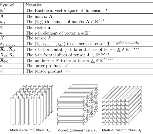
The notations used in this thesis is very similar to that presented in [38]. The important notations are presented in Table 2.1 and other notations will be introduced where they are necessary.

2.1.2 Some notations related to 3

rd

order tensor

We recall some notations related to 3rd _{tensor X ∈ R}I×J ×T from [38] which are used in later parts.

1. Fibers

Fibers are the higher order analogue of matrix rows and columns. A fiber is defined by fixing every index but one. A matrix column is a mode-1 fiber and a matrix row is a mode-2 fiber. Third-order tensors have column, row, and tube fibers, denoted by x:jt, xi:t, and xij:, respectively. Fibers are always assumed to be column vectors.

(20)

Table 2.1: List of important notations. Symbol Notation

RI The Euclidean vector space of dimension I.

A The matrix A.

aij The (i, j)-th element of matrix A ∈ RI×J.

a The vector a.

ai The i-th element of vector a ∈ RI.

X The tensor X

xd1d2...dN The (id1, id2, . . . , idN)-th element of tensor X ∈ R

d1×d2×...×dN Xi::, X:j: The i-th horizontal, j-th lateral slices of tensor X ∈ RI×J ×T

X::t, Xt The t-th frontal slices of tensor X ∈ RI×J ×T

X(n) The mode-n of N -th order tensor X ∈ RI×J ×T

◦ The outer product “◦” ⊗ The tensor product “⊗”

Figure 2.1: Fibers of a 3rd_{-order tensor [38].}

2. Slices

Slices are two-dimensional sections of a tensor, defined by fixing all but two indices. Figure 2.2 shows the horizontal, lateral, and frontal slides of a third-order tensor X , denoted by Xi::, X:j:, and X::t, respectively.

3. Mode-n matricization

The mode-n matricization of a 3rd _{tensor X ∈ R}I×J ×T is denoted by X(n) and

arranges the mode-n fibers to be the columns of the matrix. The following example of 3rd _{tensor X ∈ R}3×4×2 _{may help ones to have a better understanding about}

mode-n matricization and its relation to slices.

Let the frontal slices X1 (X::1) and X2 (X::2) of X ∈ R3×4×2 be as in Figure 2.3.

(21)

Figure 2.2: Slices of a 3rd_{-order tensor [38].}

Figure 2.3: The frontal slices of tensor [38].

Figure 2.4: The three mode-n of tensor [38].

2.1.3 Real vector space

For the sake of simplicity, we introduce an intuitive version of real vector space from [70]. Ones whose interested in mathematical definition may referred to several stand algebra books, for example [4, 10], etc.

Definition 1 A vector space V over R, or a real vector space V, is a set of objects, known as vectors, together with vector addition “+” and multiplication of vectors by element of R, and satisfying the following properties:

• (VA1) For every x, y ∈ V, we have x + y ∈ V.

(22)

• (VA3) There exists an element 0 ∈ V such that for every x ∈ V, we have x + 0 = 0 + x = x.

• (VA4) For every x ∈ V, there exists −x ∈ V such that x + (−x) = 0. • (VA5) For every x, y ∈ V, we have x + y = y + x.

• (SM1) For every α ∈ R and x ∈ V, we have αx ∈ V.

• (SM2) For every α ∈ R and x, y ∈ V, we have α(x + y) = αx + αy. • (SM3) For every α, β ∈ R and x ∈ R, we have (α + β)x = αx + βx. • (SM4) For every α, β ∈ R and x ∈ R, we have (αβ)x = α(βx). • (SM5) For every x ∈ V, we have 1x = x.

Note that the elements α, β, γ ∈ R discussed in (SM1)-(SM5) are known as scalars. Multiplication of vectors by elements of R is sometimes known as scalar multiplication.

2.1.4 _{Vector spaces R}

d1×d2×...×dN

The following definition of vector spaces Rd1×d2×...×dN _{is cited from [21]} Definition 2 Let Rd1×d2×...×dN _{be the set of all N -way array of size d}

1 × d2 × . . . ×

dN, Rd1×d2×...×dN is a vector space of dimension d1d2. . . dN together with the following

operations • Addition

A + B := C, where cd1d2...dN = ad1d2...dN + bd1d2...dN (2.1) for all A, B ∈ Rd1×d2×...×dN_.

• Scalar multiplication

λA := B, where bd1d2...dN = λad1d2...dN, (2.2) for all A ∈ Rd1×d2×...×dN _{and λ ∈ R.}

2.2 What is Tensor?

Tensor have been widely studied in various fields including mathematics, physics, engineer-ing and have became a trend in data minengineer-ing and data analytics as the rapidly increasengineer-ing of big data. But when reviewing papers and application works, we saw that the definition of tensor in some papers are somewhat vague. For example the term “a N -way data” is often referred to “a Nth-order tensor” or these two terms are used exchangeably. Also, when looking for documents with key word “tensor”, ones may see some terms related to “tensor”, for instance “metric tensor”, “stress tensor”, “Riemann curvature tensor”. To

(23)

answer the question “what is tensor?” and which “definition” we should be studied and applied in our research scope, we looking for the answer in the popular papers, books and research documents related to tensor.

Very clearly answers for the above questions can be found in [21]:

“Even though tensors are well-studied objects in the standard graduate mathematics curriculum [4, 25, 36, 42, 58] and more specifically in multilinear algebra [10, 30, 49, 55, 66], a “tensor” continues to be viewed as a mysterious object by outsiders. We feel that we should say a few words to demystify the term.

In mathematics, the question “what is a vector?” has the simple answer “a vector is an element of a vector space” in other words, a vector is charac-terized by the axioms that define the algebraic operations on a vector space. In physics, however, the question what is a vector? often means “what kinds of physical quantities can be represented by vectors?” The criterion has to do with the change of basis theorem: an n-dimensional vector is an “object” that is represented by n real numbers once a basis is chosen only if those real numbers transform themselves as expected when one changes the basis. For exactly the same reason, the meaning of a tensor is obscured by its more restrictive use in physics. In physics (and also engineering), a tensor is an “object” represented by a k-way array of real numbers that transforms ac-cording to certain rules (cf. (2.2)) under a change of basis. In mathematics, these “transformation rules” are simply consequences of the multilinearity of the tensor product and the change of basis theorem for vectors.”

Similar discussions also can be found in [38, 46]. In many documents, term “3rd _order

tensor” (or “3-way tensor”) is identical with the 3-way array A which is indeed a repre-sentation of tensor X when the bases are fixed as point out in later section 2.3. In our understanding, the reasons of this situation are formal definition of tensor and related properties in multilinear algebra are complicated and many common used results in data mining can be stated without introducing arrays of coordinates as point out in [19,38,41].

2.3 Tensor and CP-decomposition

In this section, we give definition of tensor and summary some important results from [21,46]. Ones who interested in tensor, tensor product of vector spaces and related results may referred to several papers such as [19, 21, 47, 69] and standard algebra books [4, 10, 21, 25, 30, 36, 42, 49, 55, 58, 66].

Definition 3 Let V1, V2, . . . , VN be real vector spaces of dimensions d1, d2, . . . , dN,

respec-tively, tensor product space V1⊗ V2 ⊗ . . . ⊗ VN is vector space of dimension d1d2. . . dN;

(24)

When we fix a choice of basis {en_d_in|din = 1, 2, . . . , dn}, for Vn, respectively, then X has coordinate representation X = d1 X d_i1=1 . . . dN X d_iN=1 xd_i1...d_iNe1d_i1 ⊗ . . . ⊗ e N d_iN. (2.3)

The coefficients form a N -way array, A_{∈ R}d1×...×dN_{. Also, element of an d}

n-dimensional

vector space Vn may be represented by an dn-tuple of numbers in Rdn up to a choice of

basis, for n = 1, 2, . . . , N [21].

Before giving the formulation of CP-decomposition, we summarize results from [21] which may give insight view about the relations among some related terms such as “tensor”,“N -way array”, “tensor product”, “outer product”, etc., and the first imagi-nation about CP-decomposition (or outer-product decomposition of a tensor).

Let Rd1 ⊗ Rd2⊗ . . . ⊗ RdN _{be the tensor product of the vector spaces R}d1_{, R}d2_{, . . . , R}dN and let φ be the Segre map which is a multilinear such that

φ : Rd1 × Rd2

× . . . × RdN

−→ Rd1×d2×...×dN _(2.4) (x1, x2, . . . , xN) 7−→ φ(x1, x2, . . . , xN) = X ,

where the (id1, id2, . . . , id1)-th element of X is defined as

xi_d1i_d2...i_d1 = x1i_d1x2i_d2. . . xN i_dN. (2.5)

From the universal property of tensor product we have a unique linear map θ such that the diagram in Figure 2.5 commutes, i.e,

φ((x1, x2, . . . , xN)) = θ(⊗((x1, x2, . . . , xN))) = θ((x1⊗ x2⊗ . . . ⊗ xN)), (2.6)

for all (x1, x2, . . . , xN) ∈ Rd1 × Rd2 × . . . × RdN. In other word, we have φ = θo⊗, where

“θo⊗” is composite function.

Figure 2.5: Commutative diagram [21].

Note that result of Segre map in Equation 2.5 can be write in form of outer product such that φ((x1, x2, . . . , xN)) = x1◦x2◦. . .◦xN, where “◦” is the outer product of vectors.

Equation 2.6 implies that

(25)

Furthermore, θ is a vector space isomorphism since dim(Rd1 _{⊗ R}d2 _{⊗ . . . ⊗ R}dN_{) =} dim(Rd1×d2×...×dN_{) = d}

1d2. . . dN. It implies that tensor product of vector x1⊗ x2⊗ . . . ⊗

xN and the N -way array X = φ((x1, x2, . . . , xN)) = x1 ◦ x2 ◦ . . . ◦ xN are equivalent

objects which belong to equivalent vector spaces Rd1 _{⊗ R}d2_{⊗ . . . ⊗ R}dN _{and R}d1×d2×...×dN_, respectively. Such equivalences allows us to not distinguish between these two spaces, and both X _{∈ R}d1 _{⊗ R}d2 _{⊗ . . . ⊗ R}dN _{and θ(X ) ∈ R}d1×d2×...×dN _{can be called tensor.}

Such results provide great advantages for data mining applications related to N -way array data because N -way array (consider as element of Rd1×d2×...×dN_{) may provide nature} and compact representation for data and target problem may be solve using tensor space model based methods [3, 13, 17, 34, 38, 50, 56, 59, 69]. From now on, we only focus on the special case of 3-way tensors which is indeed 3 way arrays in RI×J ×T _{because it is enough}

for understanding the content of later parts with notice that many important results are originally proved on RI⊗ RJ

⊗ RT_.

Rank-1 tensor or decomposable tensor is a special kind of tensor and is necessary to understand CP-decomposition [21, 38].

Definition 4 A 3rd_{-order tensor X ∈ R}I×J ×T is of rank one if it can be written as the outer product of 3 vectors, i.e.,

X = a ◦ b ◦ c, (2.8)

where a ∈ RI_{, b ∈ R}J _{and c ∈ R}T_.

CP-decomposition is used to decompose a tensor into a sum of component rank-one tensors [19, 38]. Theoretically, any tensor X can be decomposed (non uniquely) into a linear combination of decomposable tensors or in other words, given a tensor X ∈ RI×J ×T, we can find ar ∈ RI, br ∈ RJ and cr ∈ RT such that

X = R X 1 λrar◦ br◦ cr, (2.9) where ar∈ RI, br ∈ RJ and cr ∈ RT.

Elementwise, equation 2.9 is written as

xijt = R X r=1 λraribrjcrt, (2.10) for i = 1, 2, . . . , I, j = 1, 2, . . . , J , t = 1, 2, . . . , T and r = 1, 2, . . . , R. CP-decomposition of a 3rd-order tensor is illustrated in Figure 2.6

Matrices A = [a1, a2, . . . , aR] ∈ RI×R, B = [b1, b2, . . . , bR] ∈ RJ ×Rand C = [c1, c2, . . . , cR] ∈

RT ×R are called component matrices.

There are some kind of ranks defined on tensors, the most common ones called CP-rank, outer product rank or in short rank(.) [21, 38].

Definition 5 The rank of a tensor X , denoted rank(X ), is defined as the smallest number R of rank-one tensors that generate X as their sum.

(26)

Figure 2.6: CP decomposition of a third order tensor [38].

For a 3rd _{order tensor X ∈ R}I×J ×T_{, the lower and upper bounds of number R are}

max{I, J, T } and min{IJ, J T, IT }, respectively. Or in other words, we have the fol-lowing inequality

max{I, J, T } ≤ R ≤ min{IJ, J T, IT } (2.11) For detail about the bounds of tensor rank, ones may refer to some documents [20, 35, 38, 40], etc.

Another important remark is that in Equation 2.9, we see that for any 3rd_{-order tensor}

X ∈ RI×J ×T _{can be decomposed into a linear combination of decomposable tensors but}

we did not see how to find such combination for a given tensor. In our point of view, there is no available model to find an exactly decomposition for a given tensor. Generally, CP-decomposition is used to determine the feasible solution region for the approxima-tion problems. And based on the purpose of the approximaapproxima-tion problems, the objective functions are constructed and are solved to find the optimal solution/solutions on the determined feasible solution region. The class of models follow this procedures is called PARAFAC family and is presented in Section 2.4.

2.4 PARAFAC family

PARAFAC family consists of PARAFAC model and other models, which have relaxed the restrictions enforced by a PARAFAC model to capture data-specific structures [3]. The simplest version of PARAFAC model is R-component PARAFAC model. Given a tensor X and a number R, R-component PARAFAC model used to find a linear combination of R-decomposable tensors which is best approximates the given tensor X [3,14,15,20,21,32, 37, 38]. In other words, R-component PARAFAC model find three component matrices A = [a1, a2, . . . , aR] ∈ RI×R, B = [b1, b2, . . . , bR] ∈ RJ ×R and C = [c1, c2, . . . , cR] ∈

RT ×R by solving the following optimization problem

min A∈RI×R_,B∈RJ ×R_,C∈RT ×RkX − R X r=1 ar◦ br◦ crkF, (2.12)

where F is Frobenius norm.

Note that component matrices A, B, and C are determined uniquely up to a permu-tation and scaling of columns [3]. Permupermu-tation of column mean that if

(27)

is an optimal solution of optimization 2.12 and σ is a permutation on {1, 2, . . . , R} such that σ(1, 2, . . . , R) = (σ(1), σ(2), . . . , σ(R)) (2.13) then {A0 = [aσ(1), . . . , aσ(R)], B 0 = [bσ(1), . . . , bσ(R)], C = [cσ(1), . . . , cσ(R)]}

is also an optimal solution. And scaling of columns mean that

{A = [α1a1, . . . , αRaR], B = [β1b1, . . . , βRbR], C = [γ1c1, . . . , γRcR]}

with {αr, βr, γr∈ R|αrβrγr = 1, r = 1, 2, . . . , R} is also an optimal solution of optimization

problem 2.12.

To avoid the scaling solutions which may make the problem become more complicated, the result of optimization problem 2.12 is usually normalized and the optimization problem is reformed as follows min A∈RI×R_,B∈RJ ×R_,C∈RT ×RkX − R X r=1 λrar◦ br◦ crkF, (2.14) where {kark = kbrk = kcrk = 1|r = 1, 2, . . . , R}.

Although there is no model can find the exactly number R for a given tensor, several extension models of PARAFAC can be used to determine an appropriate number R by capturing data-specific structures [3]. Because extensions of PARAFAC are complicated and determining an appropriate number R for tensor data requires additional background, we leave those models as a future research and just list some popular models and their important characteristics in Table 2.2.

Table 2.2: Models in PARAFAC family [3].

Model name Mathematical formulation Handles rank-efficiency

Extend to N -way array PARAFAC xijt=PR_r=1aribrjcrt+ eijt No Yes

PARAFAC2 Xt= AtDtBT + Et No Yes

S-PARAFAC xijt=PR_r=1ar(i+sjr)brjcrt+ eijt No Yes

PARALIND Xt= AHDtBT + Et Yes Yes

cPARAFAC xijt=PR_r=1aribr(j−θ)cθrt+ eijt No Yes

From literature reviews, we see that applications of PARAFAC model on 3rd_-order

tensor usually consist of two stages: firstly, assuming that data have multiway structure and representing the data in form of 3rd-order tensors; then, PARAFAC model is employed to carry out three component matrices which can be understood as a new representation with certain multiway structure [3, 11, 20, 38]. Note that certain multiway structure in

(28)

this case mean that data can represented in form of a 3-order tensor which is then can be represented in CP-decomposition form.

Furthermore, when working with 3rd_{-order tensor, the number of elements that we have}

to store and manipulate is larger and rapidly increasing when the size of ways increase. It is also important to find a new representation which requires less storage memory like CP-decomposition form. For example, when working with a 3rd_{-order tensor X ∈ R}I×J ×T_{, we}

have to store and manipulate totally IJ T elements while working with R-component CP-decomposition, ones only need to concern R(I +J +T ) elements. As point out in literature reviews [20,29,38], finding good approximation with small R have been widely studied and numerous fast and efficient algorithms have been proposed, improved and implemented on popular softwares (for example MATLAB), tensor decomposition models (in particularly, PARAFAC model) have become promising solution to handle the multiway array data.

(29)

Chapter 3 CP-decomposition based temporal

link prediction on open bipartite

networks evolve over time

The first part of this chapter present necessary concepts related to temporal link predic-tion, open bipartite networks and an introduction to temporal link prediction on bipartite networks. Then the second part provides the related works need to understand the pro-posed temporal link prediction method for open bipartite networks. In the third part, the proposed method is presented. Finally, discussions and future works is given in the fourth part.

3.1 Introduction

The temporal link prediction is a common problem for data which is assumed to have the underlying periodic structure. The problem of temporal link prediction can be summa-rized as follows

Definition 6 Given link data for times 1 through Tth_{, temporal link prediction is the}

problem of predicting the links at time (T + 1)th.

Of course this is a general problem and can be found in many kinds of data. In this chapter, we restrict the problem on one special kind of data which can be represented by bipartite networks whose links evolve over time.

Definition 7 Bipartite networks are a common type of network data in which there are two types of vertices, and only vertices of different types can be connected by links [2,26,43]. In a bipartite network that evolve over time, two sets of vertices are fixed and only the links between different kind of vertices change. Figure 3.1 is an example of bipartite networks with 5 vertices of each type.

Bipartite networks can be used to represent various kinds of structures, dynamics, and interaction patterns found in social activities [8, 22, 52, 53, 67]. For example, bipartite

(30)

Figure 3.1: An example of bipartite network that evolve over time.

network is used to represent the network consists of I authors and J conferences where each link represents the possibility that an author publishes on a conference and temporal link prediction is used to predict which authors will publish at which conferences in year (T + 1)th _{given the publication data for the T previous years [2,26]; I users/group of users}

and J providers and their relations in a recommendation systems can be represented by a bipartite network [67]; Another example is the bipartite network consists of I patient groups and J drugs with the links represent the adverse effect of drugs.

In real applications, we can face some special bipartite networks with common situation that new vertices may join network at time Tth and may link to other vertices at time (T + 1)th_{. There are numerous examples about such kind of networks. For example, when}

consider a recommendation system, new users/group of users appear and may interest or use service of providers in next time points; also in drug side effect example, new drugs are launched and may have adverse effect on patient groups in the future; etc.

For simplicity, let call such networks by open bipartite networks to distinguish from bipartite networks without new added vertices. We define such kind of networks as in Definition 8 and give illustration in Figure 3.2.

Definition 8 An open bipartite network is a bipartite network in which new subjects may join the network at time T and may link to objects at time (T + 1)th.

Figure 3.2: An example of open bipartite network that evolve over time.

Several temporal link prediction methods have been proposed for bipartite networks [2, 26] but in our knowledge, no temporal link prediction method proposed to deal with problem on open bipartite networks. In our point of view, temporal link prediction on open bipartite networks is challenging because it is difficult to learn how new vertices will link to

(31)

other vertices and how new added vertices effect links among previous vertices at time (T + 1)th_{. To do temporal link prediction on open bipartite networks, we extend temporal link}

prediction method using CP-decomposition in [2, 26] to address temporal link prediction in open bipartite networks in which new vertices of type-1 may join networks at time Tth.

3.2 Related works

Temporal link prediction methods for bipartite networks assume that link data have an underlying periodic structure and apply time series techniques to predict future links [2, 5,23,26,67]. Almost traditional methods apply time series techniques directly on the link-data to predict future links. This schema is simple in implementation but have limitations such as high complexity, memory consuming and difficulty in exploiting the natural three-dimensional structure of temporal link data. Recently, temporal link prediction method using CP-decomposition were proposed and shown its power in exploring the structure of data, requiring less memory and giving outperformed experimental results comparing with the traditional methods [2, 26]. Because the proposed method for open bipartite networks can be seen as an extension of the method in [2,26], understanding the key ideas of the method proposed in [2, 26] is necessary.

3.2.1 Temporal link prediction using CP-decomposition

In the method proposed in [2, 26], a 3rd_{-order tensor is used to represent the link}

informa-tion data; CP-decomposiinforma-tion employed to explore the three dimensional structure of data; and the link information in the next time point is predicted using temporal forecasting techniques.

Figure 3.3 gives an illustration of consisting steps in this method.

Figure 3.3: Illustration of temporal link prediction method proposed in [2, 26]. The method can be summarized as follows

(32)

• Step 1: Data representation

The data is organized as a 3rd_{-order tensor X of size I × J × T , where x}

ijt represents

weight of the link between type-1 vertex ith and type-2 vertex jth at time tth. • Step 2: CP-decomposition

Carry out CP-decomposition method to get three-component matrices:

A = [a1, a2, . . . , aR] ∈ RI×R, (3.1)

B = [b1, b2, . . . , bR] ∈ RJ ×R, (3.2)

C = [c1, c2, . . . , cR] ∈ RT ×R. (3.3)

where ar ∈ RI, br ∈ RJ and cr ∈ RT, such that

X = R X 1 λrar◦ br◦ cr. (3.4) In Equation 3.4, {ar|r = 1, 2, . . . , R}, {br|r = 1, 2, . . . , R} and {cr|r = 1, 2, . . . , R}

are the type-1 vertex, type-2 vertex and time factors, respectively. Furthermore, kark = kcrk = kcrk = 1 and are obtained by normalizing the result from the

following optimization problem

min ar,br,cr = kX − R X r=1 ar◦ br◦ crk22, (3.5) and λr = karkkbrkkcrk, for r = 1, 2, . . . , R.

• Step 3: Temporal forecasting

Using assumption that time factors inherits the underlying periodic properties of data, we can predict value of time factors at time (T + 1)th_{, denoted by γ}

r, from

elements of vector cr = (cr1, cr2, . . . , crT) and the links of network at time (T + 1)th

by using temporal forecasting method as follows

Step 3.1: Predict value of time factors at time (T + 1)th from its values at T previous time.

The temporal profiles are captured in the vectors cr, r = 1, 2, . . . , R. Different

components may have different trends, for example, they may have increasing, de-creasing, or steady profiles. For each time factor vector r, its value at time (T + 1)th is estimated by γr = 1 T0 T X t=T −T0−1 crt, (3.6)

(33)

Alternatively, we can use the temporal profiles computed by CP-decomposition as a basis for predicting the scores in future [16].

Step 3.2: Predict the links of network at time (T + 1)th_.

We define the similarity score for type-1 vertex ith_{and type-2 vertex j}th_{using results}

from R-component CP model in Equation 3.4 and results in Step 3.1 as the (i, j) entry of the following matrix

XT +1 = R

X

r=1

λrγ1ar◦ br, (3.7)

or in other words, weight of links between type-1 vertex ith and type-2 vertex jth at time (T + 1)th _is x(T +1)ij = R X r=1 λrγraribrj, (3.8) for i = 1, 2, . . . , I and i = 1, 2, . . . , J .

3.3 The proposed method

In this section, we present a proposed method to predict the weights of links at time (T + 1)th _{of an open bipartite network whose the node set consists of I type-1 vertices}

and J type-2 vertices, and N new vertices of type-1 join network at time T . The pro-posed method was presented at ACIS2014 in December 2014. For the sake of an easy understanding and clear presentation, we revised some parts from the paper at ACIS2014 where the key ideas and contributions are the same.

3.3.1 Problem formulating

The method proposed in [2, 26] work for bipartite networks when the weights of all links through T previous time points are given. The key idea is to employ CP-decomposition the weight into three separated factors, each fluctuates independently from others. From this assumption, it is clear that if we known the value of time factors at time (T + 1)th, then the weights of links at time (T + 1)th _{can be found by combining the values of time}

factors at time (T + 1)th _{with values of vertex factors of type-1 and type-2. Furthermore,}

as time factors are assumed to be inherited the underlying structure of weight data, it allows to predict the values of time factors at time (T + 1)th _{from values of time factors}

in T previous time points. The method works without any addition information than weights of links in T previous time points.

Considering the problem of predicting the weights of links at time (T + 1)th _{of an open}

bipartite networks whose a new vertex of type-1 join networks at time T and may link to vertices of type-2 at time (T + 1). Furthermore, it may also have effect on the fluctuations of weights on the whole networks though the structure of networks is changed. Then, it is easy to see that the main challenges/tasks in such problem are

(34)

• to learn the effect of new vertex of type-1 on the fluctuations of weights on the whole networks,

• and to predict the weights at time (T + 1)th_.

If we employ the same assumptions, apply CP-decomposition to separate weights of links into 3 factors and predict the values of time factors as method in [2, 26], then we only have to predict the values of type-1 vertices factors corresponding to new vertex of type-1 in order to predict the weights at time (T + 1)th. Without additional information about or related to type-1 vertex factors, we can not predict the values corresponding to new vertex. Our solution for this task is to collect additional information of all type-1 vertices and learn a function which can predict values of type-1 vertex factors from the additional information and use to predict values of type-1 factors corresponding to new vertex. In case N new vertices of type-1 join network at time T , we use the function to predict all corresponding values of type-1 vertex factors. In other words, values of type-1 factors corresponding to new vertices are learned form additional information.

This schema implies that the values of factors corresponding to new vertices do not effect on learning the values of time factors corresponding to time (T + 1)th, then they do not effect on the weights of links between other vertices of type-1 and vertices of type-2. Also the proposed method is in fact the same with the method in [2, 26] when no new vertex join the networks.

The input and output of the proposed temporal link prediction method can be summa-rized as in Algorithm 1.

Algorithm 1: Temporal link prediction on an open bipartite network Input:

1. A set of information of I type-1 vertices S = {si|si ∈ RP, i = 1, 2, . . . , I}.

2. A set of information of N new vertices of type-1 Q = {q_n|q_n_{∈ R}P_{, n = 1, 2, . . . , N }.}

3. A weight tensor X ∈ RI×J ×T_{, where the (i, j, t)-th element x}

ijt is the weight

corresponding to link between type-1 vertex ith and type-2 vertex jth at time tth_{, for i = 1, 2, . . . , I, j = 1, 2, . . . , J and t = 1, 2, . . . , T .}

Output: A matrix XT +1 ∈ R(I+N )×J, with x(T +1)ij is the predicted information of

link between type-1 vertex ith _{and type-2 vertex j}th _{at time (T + 1)}th_{, for}

i = 1, 2, . . . , I, I + 1, . . . , I + N and i = 1, 2, . . . , J .

3.3.2 Assumptions

(35)

• Assumption 1: When no vertices join network, weights data have underlying periodic structure or in other words, the weights at time (T + 1)th _{can be predict}

from weights through T previous time points.

• Assumption 2: Information of vertices of type-1 is available and encoded in form of vectors in RP_{, P is a non-negative integer number.}

• Assumption 3: For each type-1 vertex factor ar, we can learn a function fr such

that ari = fr(si), where si is information of type-1 vertex ith.

3.3.3 Method

The assumptions in Section 3.3.2 are employed to construct a temporal link prediction method as follows

• Step 1: Data representation

The weights of links through T time points are organized as a 3rd-order tensor X of size I × J × T , where xijt represents weight of the link between type-1 vertex ith

and type-2 vertex jth _{at time t}th_.

Information of I type-1 vertices is represented in form of a matrix S ∈ RI×(P +1)_,

where the ith row is the row vector (1, si1, . . . , siP), for i = 1, 2, . . . , I.

Information of N new vertices of type-1 is represented in form of a matrix Q ∈ RN ×(P +1), where the nth row is the row vector (1, qn1, . . . , qnP), for n = 1, 2, . . . , N .

• Step 2: CP-decomposition

Carry out CP-decomposition method to get three-component matrices:

A = [a1, a2, . . . , aR] ∈ RI×R, (3.9)

B = [b1, b2, . . . , bR] ∈ RJ ×R, (3.10)

C = [c1, c2, . . . , cR] ∈ RT ×R. (3.11)

where ar ∈ RI, br ∈ RJ and cr ∈ RT, such that

X =

R

X

r=1

λrar◦ br◦ cr. (3.12)

• Step 3: Predict the values of type-1 vertex factors corresponding to new vertices In this works, we assume that functions fr is linear or in other words, for each r,

we have fr(si) = αr0 + P X p=1 αrpsip, (3.13) for i = 1, 2, . . . , I.

(36)

For each function fr, we use least square method [33] to estimate vector αr =

(αr0, αr1, . . . , αrP)T ∈ RP +1 as follows

αr = (STS)−1STar, (3.14)

where ST is transpose matrix of S. For each new type-1 vertex n and each type-1 vertex factor, we find the corresponding value

s0_rn = αr0+ P X p=1 αrpsip, (3.15) for n = 1, 2, . . . , N and r = 1, 2, . . . , R.

Concisely, we can found matrix α = [α1, α2, . . . , αR] ∈ RR×(P +1) such that

α = (STS)−1STA, (3.16)

and then find a matrix S0 such that

S0 = Qα, (3.17)

where the (r, n)th _{element of S}0 _{is indeed s}0

rn in Equation 3.15.

For each r, we form column vector dr∈ RD, where D = I + N , such that

dr= (ar1, . . . , arI, s 0 r1, . . . , s 0 rN) T_. _(3.18)

Note that forming vectors dr only help to make the computational procedure in

later steps more concisely. • Step 4: Temporal forecasting

Using assumption that time factors are inherited the underlying periodic properties of data, we can predict value of time factors at time (T + 1)th_{, denoted by γ}

r, from

elements of vector cr = (cr1, cr2, . . . , crT). Then the links of network at time (T +1)th

by combining γr, br and dr estimated from Step 3 by following procedures

Step 4.1: Predict values of time factors at time (T + 1)th _{from its values at T}

previous time.

The temporal profiles are captured in the vectors cr. Different components may

have different trends, for example, they may have increasing, decreasing, or steady profiles. For each time factor vector cr, its value at time (T + 1)th is estimated by

γr = 1 T0 T X t=T −T0−1 crt, (3.19)

where T0 is a prior number.

(37)

We define the similarity score for type-1 vertex dth and type-2 vertex jth using result from R-component CP model in Equation 3.12, and result from Steps 3 and Step 4.1 as the (d, j) entry of the following matrix

XT +1 = R

X

r=1

λrγrdr◦ br, (3.20)

or in other words, weight of link between type-1 vertex dth _{and type 2 vertex j}th _at

time (T + 1)th is X(T +1)dj = R X r=1 λrγrdrdbrj, (3.21) for d = 1, 2, . . . , D and i = 1, 2, . . . , J .

Note that, for d = 1, 2, . . . , I, type-1 vertex dth _{is the previous vertex i = d, and for}

d = I + 1, I + 2, . . . , I + N , type-1 vertex dth _{is the new type-1 vertex n = d − I.}

3.4 Discussions and future works

The proposed method can be applied to do temporal link prediction on open bipartite networks whose N new vertices of type-2 join networks instead of type-1 vertices since the role of type-1 vertices and type-2 vertices are the same in the proposed method.

We also point out that in the proposed method, new vertices do not effect the fluctuation of weights corresponding to links among previous vertices at time (T + 1)th_{. Furthermore,}

the proposed method is an extension of method in [2, 26], then it can be used to extend the application context in that papers.

The proposed method is an intuitive method, it should be applied to analyze datasets in order to evaluate the performance. Unfortunately, because of limited time, we have not implemented the program and tested on real datasets. We leave this task as a future work of this thesis.

In the later research, we plan to focus on the following tasks

1. Collect data and run experiments on real datasets in order to evaluate performance of the proposed method.

2. Extend the proposed method to predict the links for a period of time starting at (T + 1)th _{or in other words, for times (T + 1)}th_{, . . . , (T + L)}th_.

3. Construct temporal link prediction for open bipartite networks when the new ver-tices of type-1 and type-2 join the concerned networks at the same time.

(38)

Chapter 4 CP-decomposition based spectral

clustering

This section provides an overview of spectral clustering and suggestions to extend this method to deal with tensorial data. Firstly, we give an overview of spectral clustering including the general schema, opportunity to extend for tensor data. Also, the currents research on clustering methods for tensor data is given. Secondly, a proposed spectral clustering method namely CP-decomposition based spectral clustering is presented. Then, experiment results are analyzed to evaluate performance of the proposed method. Finally, the future plan to improve the proposed methods and suggestion to construct a versatile clustering method based on tensor space model are given.

4.1 Spectral clustering

Spectral clustering has became one of the most popular clustering algorithms [54, 64]. In this section, we present the general schema of spectral clustering and discussions that motivate us focus on studying spectral clustering and extend such methods for tensor data, though there many other clustering methods, for example, K-mean clustering, hierarchical clustering, etc.

4.1.1 General Schema of spectral clustering

Before going to present the general schema of spectral clustering, we provide an intuitive overview about spectral clustering which is summarized from technique papers [54, 64].

In applications deal with empirical data, clustering is use to identify the groups of data which have “similar behavior” and can be seen as the first attempt to learn about the structure of data. It is clear that different ways to define “similar behavior” will motivate people to construct different classes of clustering method.

One intuitive way to define the similar behavior is to assume that the T considered data points, denoted by s1, s2, . . . , sT, are embedded into a weighted similarity graph

(39)

its weight wi,j represent the “similarity” between vertex vi and vj or equivalently the

“similarity” between data point vi and sj. Then, the problem of find groups of similar

data points change to a relaxation problem that finding groups of similarity vertices in the similarity graph. The relaxation problem is easier to solve because graph and similarity graph have been studied for a long time and many powerful results have been found. By embedding the data points into a similarity graph, we can employ any techniques and results related to similarity graph to do clustering on the embed similarity graph. Finally, the result on the similarity graph can be converted to the original data space though the embedded function is clear.

The clustering methods that follow the above procedure is called spectral clustering methods. Note that “similarity” is a general notation and also there are several tech-niques to do clustering on embed similarity graph. Spectral clustering methods are dis-tinguished mainly by which similarity measures and clustering techniques on similarity graph are employed. In this thesis, we focus on symmetric similarity measure which used to constructed the embedded undirected graph with the properties that wij = wji which

is used to distinguished with other kind of graph whose wij may be different from wji.

The general schema of spectral clustering used in this thesis can be summarize as in Algorithm 2.

This schema is similar to schema in other papers [54, 64]. The only difference here is that we do not mention about any certain similarity measure as it should be chosen appropriately for each kind of data.

The matrix L in step 2 is called normalized Laplacian matrix. For other kinds of Laplacian and their applications in spectral clustering, ones are suggested to refer technical documents and survey papers [31, 64], etc.

4.1.2 Motivation and opportunity for tensor data

Before presenting the reasons that motivate us to study and extend spectral clustering methods for tensor data, we summarize two general criterias which have been used to compare clustering methods from [57] as follows

1. How easy to use the method. This criteria is usually used to compare the execution time and storage requirements of computer-oriented methods.

2. How well the performance is when applying methods to analyze data.

In our point of view, the second criteria can be used only when the evaluation criteria and purpose of the application problems are determined, and considered methods are used under same restricted conditions. Also, we suggest to consider “how easy to interpret the result” and “how easy to extend method for complex kinds of data” as parts of the first criteria when applying clustering method in data mining applications because interpret the result is a crucial steps and complex data has became a challenge in numerous real applications related to data mining.

Concerning the above criteria, we have seen reason that motivate us to focus on spectral clustering as follows

(40)

Algorithm 2: General schema of spectral clustering Input:

1. A set of T data point P = {st|t = 1, 2, . . . , T }, where st represents information of

data point tth_.

2. A similarity function S

S :P × P −→ R\(−∞, 0) (si, sj) 7−→ S((si, sj)) = wij.

3. A number K of data groups.

Output: K groups of data points G1, G2, . . . , GK such each data point st belong to

one group Gk, for t = 1, 2, . . . , T and k = 1, 2, . . . , K.

1. Construct an embedded undirected similarity graph G = (V, E) using similarity measure S.

2. Compute the similarity matrix W, where the (i, j)-th element of W is wij = S(vi, vj).

3. Define D to be the orthogonal matrix whose (i, i)-th element is the sum of elements in W’s i-th row, and compute Laplacian matrix L = D−1/2WD−1/2. 4. Compute the first K largest eigenvectors u1, u2, . . . , uK of L and form the matrix

U = [u1, u2, . . . , uK] ∈ RT ×K] by stacking the eigenvectors in columns.

5. Form a matrix Y from U by renormalizing each of U’s row to have unit norm. 6. Treating each row of Y as a vector in RK and cluster them via K-mean method. 7. Finally, assign the original point st to the the cluster k if row tth of Y was assigned

JAIST Repository: Study on tensor calculus and CP-decomposition