1 INTRODUCTION
Under todayʼs global business environment, supply chains have become more complex and uncertain because suppliers and customers of a company spread throughout the world. There is a probability that supply chains might be disrupted. Therefore, how to design and manage supply chains has become one of the most important strategy for companies to gain advantages in competition with others.
A supply chain can be viewed as a process or a network consisting of several participants. To achieve the efficiency of the whole supply chain, participants must streamline its internal processes. There are several effective production strategies as well as inventory policies such as just-in-time (JIT), make-to-order (MTO), built-to-order (BTO), and so forth. These strategies can be used to enhance the efficiency of companyʼs internal processes. For example, Toyota Motor, the inventor of the JIT production system, has become worldʼs best car maker. Dell Computer has been realizing mass customization by employing the BTO production strategy.
In addition to streamlining internal processes, a company need to collaborate with its partner to enable the entire supply chain to be more efficient and competitive. As the development of information technology, information sharing and coordination among participants have become easier than ever before. The order information of downstream customers
SIMULATION ANALYSIS OF A
JUST-IN-TIME SUPPLY CHAIN SYSTEM
XIAOHUA WANG
is one of the most important factors for making the production plan and inventory management. Advance demand information (ADI) is obtained when customers place orders in advance for a future delivery [1]. If there is ADI available, the company could adopt more flexible production policy as well as inventory control policy.
There are a number of studies dealing with the issues of production and inventory strategies as well as ADI. Several literatures have investigated the benefits of integrating ADI with pull-kanban production and inventory system using simulation [2, 3]. Sarkar and Shewchuk [4] have examined the benefits of three-stage production-inventory systems serving two customer classes with and without ADI. The researches have demonstrated that the considered system can obtain the benefits of employing ADI under the assumption settings.
However, these studies just have considered one facility problem. By contrast, this research is to investigate the performance of a supply chain consisting of a manufacturer and a supplier with JIT control philosophy. Specifically, we examine the impacts of kanban settings such as the number of production and safety kanbans, the delay coefficient of supplier kanbans on performance measures that are the average inventory and the average backorders. The results show that the supplier as well as the supply chain system can gain the benefits of adopting different production strategies with different kanban cycle settings. In other words, the supplier can employ different production strategies such as MTO, BTO, and MTS based on whether there is ADI available.
Since such system with uncertainty is very complex to analyze by using an analytical model, simulation modeling is a suitable tool for analyzing supply chains [5]. There have been a great number of literatures on analysis of supply chains and production-inventory systems by using simulation methodology [2-4, 6-8]. The studies have shown its efficiency and effectiveness.
The rest of this paper is organized as follows. Section 2 gives a briefly description of the system related to this study. Section 3 describes the simulation model and Section 4 presents the simulation results and discussions. Finally, the conclusions are presented in Section 5.
2 SYSTEM DESCRIPTION
The JIT supply chain system under consideration consists of a manufacturer and a supplier. The manufacturer produces two types of products using two parts provided by the supplier. Each product uses one part. The total daily quantity of the products is constant, but the quantity of each product is uncertain. Kanban-based control policy is used by the manufacturer, the supplier, and the transportation between the manufacturer and the supplier. The supplier may employ the MTS, BTO, and MTO strategy depending on the demand lead time which is the time interval between the order arrival and the order due date.
2.1 Kanban-based control system
JIT basically means to produce the necessary units in the necessary quantities at the necessary time [9], and it is one pillar of Toyota Production System (TPS). Kanban is a tool for implementing a JIT production or delivery system. It can be viewed as an information system which harmoniously controls the production quantities in every process [9]. As an ordering policy, that is very similar to an (R, Q) policy as well [10]. We use the kanban control policy introduced by Monden [9] and Kotani [11]. There are two types of kanbans: one is the production kanban and the other is the withdrawal kanban (or supplier kanban). The production kanban is used within process, and the withdrawal kanban is used between processes. The withdrawal kanban is called the supplier kanban if supplier own the preceding process. In this study, the number of production kanbans at the manufacturer as well as
the supplier is to be selected as experiment factor. The number of supplier kanbans is determined by a-b-c supplier kanban cycle, which means that the supplier delivers parts b times every a days with c times delay after receiving the kanban order [9, 11]. The parameter c is called the kanban delay coefficient, and it includes demand lead time for the supplier. Figure 1 shows the a-b-c supplier kanban cycle.
Figure 1: Illustration of the a-b-c supplier kanban cycle [9]. The number of the supplier kanban can be expressed as follows [11]:
Where
D: average daily demand of the part, S: safety stock of the part,
M: container capacity of the part,
: minimum integer not less than x.
This equation will be used to generate the number of the supplier kanban. 2.2 Supplier production strategies
We assume that the order information between the manufacturer and the supplier is as follows. The manufacturer sends a three-month production schedule to its parts supplier. The forecast for the remaining two months is
estimated. The information about the most recent month is a final forecast. The firm orders are determined by the supplier kanban that cannot be changed. The supplier can adopt different production strategies based on whether the supplier kanban has different ADI that is determined by the delay coefficient.
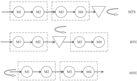
In this study, the supplier production system consists of two-stage manufacturing processes. The two parts can share the first-stage process, that is, the differences between the parts are made on the second stage. Therefore, the supplier can employ three production strategies that are the MTS, BTO, and MTO strategy. The MTS strategy is adopted if no ADI or the ADI is less than the processing time of the second stage; the BTO strategy is used if the ADI larger than the processing time of the second stage; otherwise, the MTO strategy is employed. Figure 2 shows the illustration of the strategies.
Figure 2: Illustration of the MTS, BTO, and MTO strategies. 2.3 Performance measures
goods (FG), the work-in-process (WIP), and the pipeline inventory that is the inventory on the transportation. Furthermore, the manufacturer just holds the FG inventory, while the supplier may hold the FG and the WIP inventory based on the production strategy. Raw material inventory is not considered in this research that means there is sufficient capacity available.
A backorder means that the order will wait if there is no inventory available when it arrives. It may occur at both the manufacturer and the supplier. The manufacturerʼs production line will stop if the backorder occurs. Therefore, the backorder is a crucial factor in the production and inventory system.
When a simulation run, all these inventory and backorder will be calculated. We choose the average value of these factors as performance measures in this study.
1. Total average inventory
(a) Average inventory at the manufacturer. (b) Average WIP inventory at the supplier. (c) Average finished inventory at the supplier.
(d) Average pipeline inventory from the supplier to the manufacturer. 2. Total average backorders
(a) Average backorders at the manufacturer. (b) Average backorders at the supplier. 3 SIMULATION MODEL AND EXPERIMNTS
Arena/SIMAN [12] simulation software was used for building the model and conducting the experiments.
3.1 Simulation model
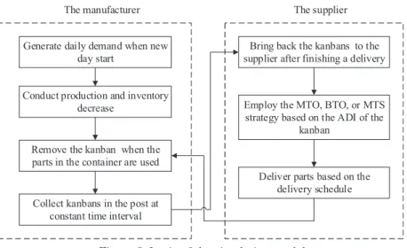
manufacturer. The main processes are shown as follows. First, the worker removes the supplier kanban and places it in the kanban post when using the first part of the container at the manufacturer. Second, the kanban in the post is collected at a constant interval. The drivers of the supplier bring the kanban back when they deliver the parts at a predetermined time. Third, the supplier calculates the due date and decides when to produce the parts. Finally, the supplier delivers the parts at determined time to the manufacturer. Figure 3 shows the logic of the simulation model.
Figure 3: Logic of the simulation model.
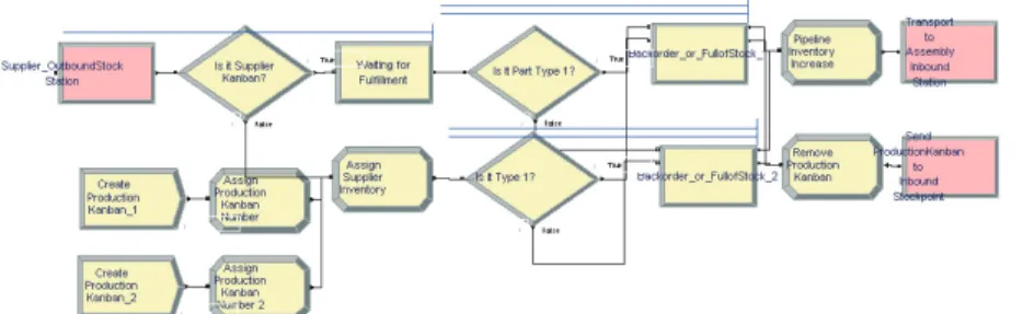
More detailed processes are necessary to realize the logic above. In the manufacturer, there are processes of the production, collecting the supplier kanbans, receiving the delivery, and so on. In the supplier, processes relating the order processing, the production, and the delivery activities are needed. It is much complicated in the simulation model. Therefore, we just take the example of the order processing at the supplier based on the MTS policy. Figure 4 shows the process in the model.
The order processing is performed at the outbound stock station of the supplier. There are two types of entities arriving: the supplier kanban and the production kanban. The former represents the order information from the manufacturer, and the latter represents the inventory information. Two entities from the manufacturer and the production line of the supplier arrive at the station module, which is a rectangle module on the left. Then, they are divided using the decide module. The supplier kanban leaves from the right exit of the module, and waits for fulfilling the order if demand lead time exists. On the other hand, the production kanban of the supplier with the products manufactured at the workstation exits from the bottom of the
decide module, and then the FG inventory at the supplier is updated. Next,
the supplier kanban and the production kanban of the supplier are forwarded based the type of parts. We use the match module to conduct the order fulfillment. That is, the number of supplier kanbans must equal to that of the production kanbans. The supplier kanbans need to wait if there are no the production kanbans at the moment. And then, fulfilled the orders which include the supplier kanbans and parts are delivered to the manufacturer. Meanwhile, the removed production kanbans are sent back to the production line. The modules on the lower left are used to create the initial production kanbans and inventory.
Several methods are used to verify the simulation model. First is to use the constant parameters as input to test the logic of the model. Second is to observe the animation when a simulation running. The animations include the plots, queues, and changes in the variables such as inventory and backorders. Figure 5 shows the variation in the number of supplier kanbans at the manufacturer. The supplier kanbans are brought to the supplier every delivery time. Between the delivery times, the supplier kanban is removed to the post when the parts in the container begin to be used.
Figure 4: Partial model for order processing at the supplier with MTS strategy.
Figure 5: The number of kanbans in the withdrawal post. 3.2 Assumptions and parameters
Assumptions are as follows. The manufacturer produces two types of products. Each product use one part provided by the supplier. The demand quantity may change daily, but the total quantity keeps constant. The supplier has enough raw material to manufacture the parts, and two parts share the partial process.
The following factors are chosen to conduct simulation experiments:
1. The number of the safety kanbans.
3. The delay coefficient of the supplier kanban.
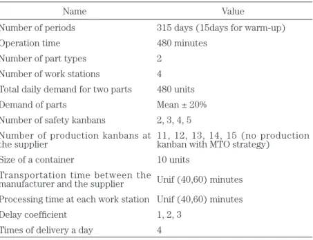
Table 1 shows the value of the factors and the parameters in detail. Table 1: Parameters for simulation experiments.
Name Value
Number of periods 315 days (15days for warm-up)
Operation time 480 minutes
Number of part types 2
Number of work stations 4 Total daily demand for two parts 480 units
Demand of parts Mean ± 20%
Number of safety kanbans 2, 3, 4, 5 Number of production kanbans at
the supplier 11, 12, 13, 14, 15 (no production kanban with MTO strategy) Size of a container 10 units
Transportation time between the
manufacturer and the supplier Unif (40,60) minutes Processing time at each work station Unif (40,60) minutes
Delay coefficient 1, 2, 3
Times of delivery a day 4
The delay coefficient, that is c, is the most important factor. It determines the supplier production strategy as well as the supply chain performance. The relationship between the delay coefficient and production lead time is shown in Figure 6.
Figure 6: Relationship between the delay coefficient and production lead time. 4 RESULTS AND ANALYSIS
In this section we analyze the results of the simulation experiments mentioned above. Section 4.1~ 4.3 investigate the performance evaluation of the system under different supplier production policies, namely MTS, BTO, and MTO, respectively. Section 4.4 compares the three different policies and discuss the benefits of the policies.
4.1 Simulation results for MTS policy
Table 2 shows a set of sample results for the system where the supplier employs the MTS production policy. As mentioned earlier, the system performance measures are average backorders and average inventory, and the inventory includes the WIP, pipeline, and FG inventory. Since the supplier employs different production policies, that is MTS, BTO, and MTO, the stock points would be different. For example, there are WIP and FG inventory with an MTS policy, but none with an MTO policy.
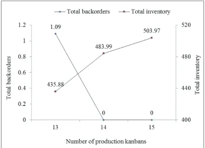
Figure 7 illustrates the variation of total backorders and total inventory with the number of production kanbans at the supplier. We just summed up the average backorders occurred at the manufacturer as total backorders
because they can make a final assembly line stop. Total inventory is the sum of all WIP, pipeline, and FG inventory. The number of production kanbans at the supplier takes the value of 13, 14, and 15, while the delay coefficient is set to 1, and the number of safety kanbans is equal to 3.
As can be seen from Figure 7 and Table 2, total inventory increases with increases in the number of production kanbans at the supplier. On the other hand, total backorders decrease, but the variation is not significant and is equal to zero when the number of production kanbans is larger than 14.
Table 2: Sample results for the MTS policy.
Number of production kanban at the supplier
13 14 15 AvgBackorderAssembly1 0.1 0 0 AvgBackorderAssembly2 0.99 0 0 Total backorders 1.09 0 0 AvgInventoryAssembly1 56.6 72.92 72.25 AvgInventoryAssembly2 53.14 67.89 68.64 Manufacturer inventory 109.74 140.81 140.89 AvgInventoryPipeline1 33.6 31.49 31.59 AvgInventoryPipeline2 32.54 31.69 31.48 Pipeline inventory 66.14 63.18 63.07 AvgInventorySupplier1 29.29 40.31 49.5 AvgInventorySupplier2 30.78 39.45 50.28 AvgWIPSupplier 99.88 100.05 100.04 AvgWIPSupplier1 50.4 49.86 50.29 AvgWIPSupplier2 49.65 50.33 49.9 Supplier inventory 260 280 300.01 Total inventory 435.88 483.99 503.97
Figure 7: Effects of the number of production kanbans with the MTS policy. 4.2 Simulation results for BTO policy
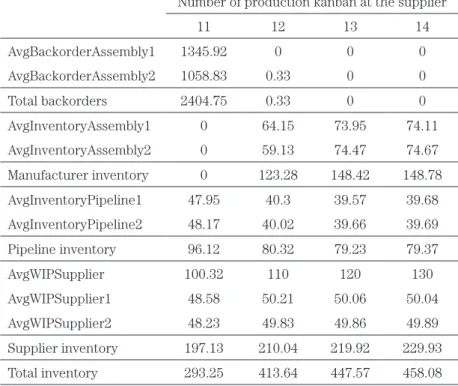
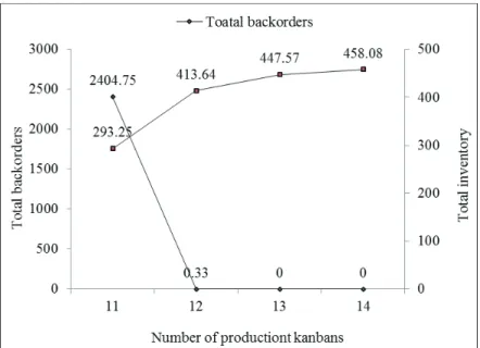
Table 3 provides a set of sample results for a system where the supplier employs the BTO production policy. It is similar to the MTS policy that average backorders and average inventory are selected as performance measures. The supplier can postpone its production to perform the BTO policy. Therefore, there is no FG inventory at the supplier. Figure 8 plots the variation of total backorders and total inventory with the number of production kanbans at the supplier. The number of production kanbans at the supplier takes the value of 11, 12, 13, and 14, while the delay coefficient is set to 2, and the number of safety kanbans is equal to 3. Like the MTS policy, total inventory increases with increasing the number of production kanbans at the supplier, while total backorders decrease.
Table 3: Sample results for the BTO policy.
Number of production kanban at the supplier
11 12 13 14 AvgBackorderAssembly1 1345.92 0 0 0 AvgBackorderAssembly2 1058.83 0.33 0 0 Total backorders 2404.75 0.33 0 0 AvgInventoryAssembly1 0 64.15 73.95 74.11 AvgInventoryAssembly2 0 59.13 74.47 74.67 Manufacturer inventory 0 123.28 148.42 148.78 AvgInventoryPipeline1 47.95 40.3 39.57 39.68 AvgInventoryPipeline2 48.17 40.02 39.66 39.69 Pipeline inventory 96.12 80.32 79.23 79.37 AvgWIPSupplier 100.32 110 120 130 AvgWIPSupplier1 48.58 50.21 50.06 50.04 AvgWIPSupplier2 48.23 49.83 49.86 49.89 Supplier inventory 197.13 210.04 219.92 229.93 Total inventory 293.25 413.64 447.57 458.08
Figure 8: Effects of the number of production kanbans with the BTO policy. 4.3 Simulation results for MTO policy
Table 4 shows a set of sample results for a system where the supplier employs the MTO production policy. We also choose average backorders and average inventory as performance measures. Since the supplier employs the MTO policy, there is no finished parts inventory at the supplier. In addition, production kanbans are not necessary with the MTO policy. On the other hand, the supplier kanbans need to wait the parts to be made, so the manufacturer has to hold more safety stock to avoid the occurrence of backorders. Therefore, we investigate the effect of safety stock on the performance measures. Figure 9 illustrates the variation of total backorders and total inventory with the number of safety kanbans. The number of safety kanbans takes the value of 2, 3, and 4, while the delay coefficient is set to 3. As can be seen from Figure 9 and Table 4, total inventory increase with increasing the number of safety kanbans, whilst total backorders decrease.
Table 4: Sample results for the MTO policy.
Number of safety Kanban
2 3 4 AvgBackorderAssembly1 212.65 0.31 0 AvgBackorderAssembly2 165.66 0.32 0 Total backorders 378.31 0.63 0 AvgInventoryAssembly1 3.35 58.8 83.48 AvgInventoryAssembly2 3.33 51.39 85.48 Manufacturer inventory 6.68 110.19 168.96 AvgInventoryPipeline1 49.71 49.7 49.71 AvgInventoryPipeline2 48.78 49.52 49.45 Pipeline inventory 98.49 99.22 99.16 AvgWIPSupplier1 100.3 100.02 100.66 AvgWIPSupplier2 98.72 100.01 99.59 Supplier inventory 199.02 200.03 200.25 Total inventory 304.19 409.44 468.37
4.4 Comparison of simulation results
Since it is not desirable that the production line stops, so the occurrence of backorders should be avoided as possible. However, contrary to daily demands of 480, one percent of backorders, that is around five units, should be reasonable. Therefore, we choose a scenario from three policies where the backorders are less than five to compare the benefits. Table 5 gives the results, and Figure 10 plots the variation of inventory with each policy. Figure 10 shows that the total inventory for the MTO policy are the lowest comparing those for the BTO and MTS policies. It indicates that the MTO policy is the best for the supply chain system considered in this study. However, since the system consists of the supplier and the manufacturer, we should give further discussion for each in detail. The inventory system can be simply divided into three echelons: manufacturerʼs inventory, pipeline inventory, and supplierʼs inventory, respectively. We do not distinguish between the WIP and FG inventory in our study. For example, the supplier inventory is the sum of the WIP and FG inventory at the supplier. All the results shown in Tables and Figures are the average values of the performance measures.
For the supplier inventory, it is similar to the total inventory that benefit from the MTO policy is superior to that from the BTO and MTS policies, and the BTO policy is better than the MTS policy. On the other hand, for the manufacturerʼs inventory, there is almost no difference among three policies. It means that the supplier production policy would not affect the performance of the manufacturer under the assumption of this study. Because the supplier production policies are based on the delay coefficient of the supplier kanban cycle, we can say there is no significant negative effect on the performance of the manufacturer in which longer delay coefficient is employed.
As mentioned earlier, the pipeline inventory is those on the way of delivering to the manufacturer. The transportation time between the supplier
and the manufacturer cannot be neglected, so the effect of the pipeline inventory also needs to be considered. It is can be seen from Figure 10, the pipeline inventory shows an increasing trend by using the MTS, BTO, and MTO policies, respectively. In this research, the transportation time and the processing time at the supplier are uncertain. The truck should have enough time to avoid delivering delay because that may cause backorders. Since the supplier begins the production after the supplier kanban arriving under the MTO policy, the uncertainty must be more significant than the BTO and MTS policies. In turn, higher pipeline inventory occurs.
However, the total inventory has improved when the supplier change the production policy from the MTS to the BTO to the MTO policy. From the viewpoint of the supply chain system, the MTO policy should be employed.
Table 5: Comparison of three policies.
MTS BTO MTO
Manufacturer inventory 109.74 123.28 110.19
Pipeline inventory 66.14 80.32 99.22
Supplier inventory 260 210.04 200.03
Figure 10: Comparison of MTS, BTO, and MTO policies. 5 CONCLUSIONS
In this study, we have investigated the performance evaluation of the JIT supply chain system by using a simulation-based approach. The system is composed of a manufacturer and a supplier. The supplier provides the parts to the manufacturer with JIT philosophy that is realized by the kanban control mechanism. The kanbanʼs parameter settings, especially the delay coefficient of the supplier kanban, would have significant effects on the supplier production strategies, in turn, influence the system performance measures that are total inventory and total backorders. Therefore, we examined how the supplier production strategies that are the MTS, BTO, and MTO affected the system performances. From the results of simulation and the discussion earlier, we could conclude that when the supplier adopt the MTO policy that means the supplier kanban with the large delay coefficient, the system have the best performance. Specifically, the benefit is almost derived from
the inventory reduction of the supplier. In other words, the supplier could gain the greatest benefit of extending the supplier kanban cycle, while the manufacturer is almost not affected by the kanban settings. It indicates that the participants in such supply chain system should collaborate with each other to obtain the greatest benefit for the whole supply chain.
However, because the results are based on the assumptions of this study, some limitations exist. For example, the number of supplier kanbans for two parts is set to constant values in the scenarios. Also, we do not examine the impact of processing time and transportation time with uncertainty on the system performance. Such limitations should be examined in the future research.
REFERENCES
1. Özer, Ö. and W. Wei, Inventory control with limited capacity and
advance demand information. Operations Research, 2004. 52(6):
988-1000.
2. Krishnamurthy, A. and D. Claudio, Pull systems with advance demand
information, in Proceedings of the 2005 Winter Simulation Conference, M.E. Kuhl, et al., Editors. 2005,1733-1742. Piscataway,
New Jersey: Institute of Electrical and Electronics Engineers. 3. Claudio, D. and A. Krishnamurthy, Kanban-based pull systems with
advance demand information. International Journal of Production
Research, 2009. 47(12): 3139-3160.
4. Sarkar, S. and J.P. Shewchuk, Use of advance demand information in
multi-stage production-inventory systems with multiple demand classes. International Journal of Production Research, 2013. 51(1):
57-68.
5. Jain, S., et al., Development of a high level supply chain simulation
Conference, B.A. Peter, et al., Editors. 2001,1129-1137. Piscataway,
New Jersey: Institute of Electrical and Electronics Engineers, Inc. 6. Wang, X.H. and S. Takakuwa, Module-based modeling of
production-distribution system considering shipment consolidation, in Proceedings of the 2006 Winter Simulation Conference, L.F.
Perrone, et al., Editors. 2006,1477-1484. Piscataway, New Jersey: Institute of Electrical and Electronics Engineers, Inc.
7. Nomura, J. and S. Takakuwa, Module-based modeling flow-type
multistage manufacturing systems adopting dual-card KANBAN system, in Proceedings of the 2004 Winter Simulation Conference, R.G. ingalls, et al., Editors. 2004,1065-1072. Piscataway,
New Jersey: Institute of Electrical and Electronics Engineers, Inc. 8. Wadhwa, S., et al., Effects of information transparency and
cooperation on supply chain performance: a simulation study.
International Journal of Production Research, 2010. 48(1): 145-166. 9. Monden, Y., Toyota production system: an integrated approach to
just-in-time. 4th ed. 2012, Boca Raton, FL: CRC Press.
10. Axsater, S., Inventory Control. 2nd ed. 2006, New York: Springer. 11. Kotani, S., Optimal method for changing the number of kanbans in
thee-Kanban system and its applications. International Journal of
Production Research, 2007. 45(24): 5789-5809.
12. Kelton, W.D., R.P. Sadowski, and D.T. Sturrock, Simulation with arena. 3rd ed. 2004, New York: McGraw-Hill.
![Figure 1: Illustration of the a-b-c supplier kanban cycle [9].](https://thumb-ap.123doks.com/thumbv2/123deta/5710069.1015509/4.629.90.500.260.401/figure-illustration-b-c-supplier-kanban-cycle.webp)