PAPER
A Nonlinear Approach to Robust Routing Based on
Reinforcement Learning with State Space Compression
and Adaptive Basis Construction
Hideki SATOH†, Member
SUMMARY A robust routing algorithm was developed based on reinforcement learning that uses (1) reward-weighted principal component analysis, which compresses the state space of a network with a large number of nodes and eliminates the ad-verse effects of various types of attacks or disturbance noises, (2) activity-oriented index allocation, which adaptively constructs a basis that is used for approximating routing probabilities, and (3) newly developed control space compression based on a potential model that reduces the control space for routing probabilities. This algorithm takes all the network states into account and re-duces the adverse effects of disturbance noises. The algorithm thus works well, and the frequencies of causing routing loops and falling to a local optimum are reduced even if the routing infor-mation is disturbed.
key words: robust routing, reinforcement learning, multivariate analysis, function approximation
1. Introduction
Advances in communications technologies have led not only to the Internet but also to various types of net-works such as sensor netnet-works [1] and ad hoc netnet-works [2]. To enable effective use of these networks, various dynamic routing algorithms have been developed [1], [2], [3]. However, dynamic routing problems have not been solved completely for these networks. This is be-cause they are essentially equivalent to a large-scale nonlinear control problem for a time-varying system that has a great many state variables and control in-puts. That is, not only traffic but also the network structure frequently changes, and the routing prob-lems have a dimensional state space and a high-dimensional control space because the network has a large number of nodes. As a result, it is difficult to con-struct an effective mathematical model of the network, and thus it is almost impossible to obtain the optimum solution within the allowable time. Secure and robust routing is also a difficult problem because of the grow-ing number of attacks for which countermeasures have not yet been implemented [1].
Reinforcement learning [4] has received much at-tention because it can handle various types of envi-ronments without using a mathematical model, and
Manuscript received July 23, 2007. Manuscript revised February 21, 2008.
†The author is with the Future University-Hakodate, Hakodate-shi, 041-8655 Japan.
many routing algorithms based on reinforcement learn-ing have been developed [5], [6], [7]. However, all pos-sible state spaces and control spaces are not handled in these algorithms because it is very difficult using rein-forcement learning to handle environments with a high-dimensional state space and a high-high-dimensional control space. Thus, the effectiveness of these algorithms is limited, and they frequently cause routing loops, which makes it difficult to find the optimum route. Moreover, most of these algorithms cannot take the adverse ef-fects of various types of attacks or disturbance noises into account.
A robust routing algorithm based on reinforcement learning that uses three methods has been developed to solve these problems. The first method is state space compression based on reward-weighted principal com-ponent analysis [8], which is used to extract the princi-pal elements from a large number of state variables and compress the state space. The second method is adap-tive basis construction based on activity-oriented index allocation [9], which is used to update the orthonormal basis and to approximate a control function. These two methods are effective for reinforcement learning with a high-dimensional state space environment. Their use in combination was investigated, and reinforcement learn-ing uslearn-ing them is described in Sect. 2. The third method is newly developed control space compression based on a potential model described in Sect. 3. It is used to reduce the control space for routing probabil-ities and to reduce the frequencies of causing routing loops and falling to a local optimum. The application of these three methods to routing problems using a non-linear approach is described in Sect. 3. Following a de-scription of the routing algorithm in Sect. 4, it is shown that the algorithm can identify the approximate opti-mum route even if there are attacks that disturb the routing information.
2. Reinforcement Learning in High-Dimensional Continuous State Space
Two previously developed methods, state space com-pression [8] and adaptive basis construction [9], are ef-fective in reinforcement learning for a high-dimensional state space environment. A structure of reinforcement
learning that includes both methods was investigated in detail. The structure is described and its efficiency is clarified in this section.
2.1 Reinforcement Learning
A system with reinforcement learning [4] is divided into two parts: agents and an environment. The former provide control functions, and the latter is the target system to be controlled. An agent observes the state and the reward from the environment, updates a control function accordingly, and outputs a new control input to the environment. The control function and control input are referred to as policy and action, respectively. Consider a discrete-time, continuous-state, continu-ous-action environment. Let sdef= (s1, · · · , sds)tbe the state vector, u def= (u1, · · · , udu)
t be the action vector,
and superscript t denote transposition. An implemen-tation of the actor-critic method [4], [8], which is used to perform reinforcement learning, is summarized in this section. The actor-critic method consists of two parts: an actor and a critic. Let st be the state
vec-tor at time t and ut be the action vector at time t.
The actor observes state st and decides on action ut,
which is a sample value from the conditional Gaussian distribution with density p(ut|st) defined by
p(u|s) ∼=
du Y
d=1
pd(ud|s), (1)
where pd(ud|s) is a one-dimensional conditional
Gaus-sian density function with mean µd(s) and standard
deviation σd(s).
The critic observes reward rt and updates µd(s)
and σd(s) so that discount return Rt, defined by
Rt def= ∞ X t0=0 νDR t0 rt+t0+1,
is maximized, where νDRis the discount rate (0 ≤ νDR≤ 1). The values of µd(s) and σd(s) are initially set
so that ut is distributed across the definition domain.
Thus, the critic can learn the relationships among rt, st,
and ut. As the critic progresses in the learning, µd(s)
and σd(s) are updated so that Rtbecomes larger. For
1 ≤ d ≤ du, µd(s) and σd(s) are expressed using the
following linear function approximations:
µd(s)def= N X i=0 ξdiφi(s), (2) σd(s)def= hlimit( N X i=0 ηdiφi(s)), (3)
where {φi(s)} is a basis and hlimit(·) is a monotone
increasing function such that 0 ≤ hlimit(x) < ∞ for
−∞ ≤ x ≤ ∞. The update of µd(s) and σd(s) can
be done by adjusting parameters ξd0, · · ·, ξdN, and ηd0,
· · ·, ηdN using temporal-difference (TD) learning and
the steepest descent method.
When the dimension of st is high, N , the degree
of expansion of µd(s) and σd(s), is too large to
per-form reinforcement learning. This problem, which is the so-called “curse of dimensionality,” is the most se-rious problem of function approximation and reinforce-ment learning for a high-dimensional state space. 2.2 State Space Compression Based on
Reward-Weighted Principal Component Analysis
Let us consider an environment with a high-dimensional state space. In such a case, it is difficult to perform re-inforcement learning, as explained in Sect. 2.1. A state space compression method based on reward-weighted principal component analysis (RWPCA) [8], which was developed to solve such problems, is summarized in this section.
Let xt def= (x1;t, · · · , xdx;t)
t be the state vector of
the environment at time t. The most simple solution is to perform principal component analysis (PCA) [10], which can extract the principal components from xt.
However, it is not always true that elements in xtwith
large dynamics contribute to increasing the reward. Some elements may be disturbance noises or attacks, which adversely affect the system [1].
To eliminate such adverse effects from xt and to
construct principal axes that contribute to increasing the reward, the resolution of xd;t, resd, is introduced,
which represents the importance of xd;twith respect to
increasing the reward. Consider the following multiple regression equations [10]: xd;t+1= βd0+ du X d0=1 βudd0ud0;t+ dx X d0=1 βxdd0xd0;t, (4) rt+1= b0+ du X d=1 budud;t+ dx X d=1 bxdxd;t, (5)
where b0, bud, bxd, βd0, βudd0, and βxdd0 are the partial
regression coefficients. Because it is clear that |bxd| is
proportional to the effect of xd;ton the reward and that
|βudd0| is proportional to the controllability of xd;t+1by
ud0;t, resdis set so that resd is proportional to |bxd| and
|βudd0|.
Let xRt( def
= (res1x1;t, · · · , resdxxdx;t)
t) be the state
vector weighted by the resolution and eRd be the dth
eigen vector obtained by PCA with respect to xRt.
Us-ing principal axes matrix MR
def
= [eR1, · · · , eRdx], the reward-weighted principal axes matrix MRW can be de-fined by MRW def = [diag[resd]MR] ds 1 , (6)
where ds≤ dx and [X]d1s denotes the matrix that
stused by reinforcement learning is set as
st= MRW
tx
t. (7)
Because MRWis composed of dseigen vectors that affect the reward significantly, we not only can compress the
dx-dimensional state, xt, to the ds-dimensional state,
st, but also eliminate the adverse effects of disturbance
noises from xt[8].
2.3 Adaptive Basis Construction Based on Activity-Oriented Index Allocation
Let {K(s, k)} be a multi-dimensional orthonormal ba-sis and kdef= (k1, · · · , kds)
t; k is referred to as the index
vector. Let φi(s) be defined as
φi(s)def= K(s, k), (8)
and basis {φi(s)} be a subset of {K(s, k)}, where i
is referred to as the index of the basis [9]. Let Dk
denote a set of k that is used in Eq. (8). When
Dkddef= {0, 1, · · · , Nd} and Dk is given by the Cartesian
product as Dk = Dk1× Dk2×, · · · , ×Dkds, the relation-ship between k and i can be obtained using
i = ds X d=1 kd ds Y d0=d+1 Nd0, (9) and N is given by N = ds Y d=1 (Nd+ 1) − 1. (10)
It is clear from Eq. (10) that N geometrically in-creases with respect to ds. Thus, if Dk is given by
the Cartesian product of Dkd and ds is large, N is too
large to perform reinforcement learning. If N is small, we may not obtain the required accuracy. This is the curse of dimensionality.
Adaptive basis construction is another solution to this problem. Various methods have been developed for adaptively constructing a basis function, most of which use the radial basis function (RBF) [4] and ad-just the parameters of RBF [11]. However, orthonor-mal bases are superior to non-orthogonal bases such as RBF from the viewpoint of the trade-off between N and the approximation error [12]. Thus, the activity-oriented index allocation method (AIA) [9] is used here; it adaptively constructs an orthonormal basis in accor-dance with the changes in the environment so that re-inforcement learning works well for a given N .
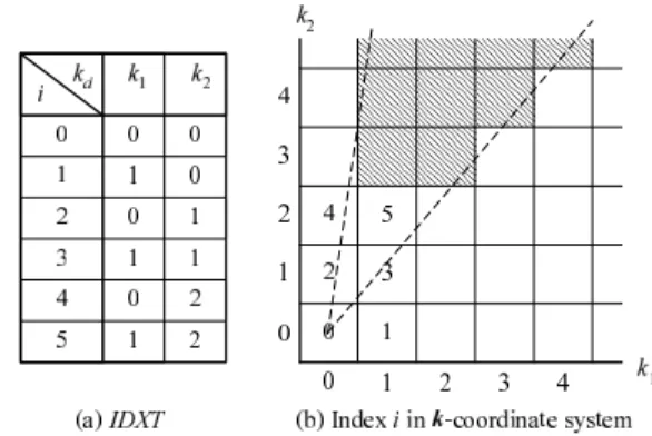
Let us introduce an index table, IDXT , defined by an (N + 1) × ds matrix to express the relationship
be-tween i and k. An example IDXT , when Dk is given by
the Cartesian product, ds= 2, N1= 1, and N2 = 2, is
shown in Fig. 1-a. Consider k1, · · ·, kdsto be the coordi-nates with respect to a rectangular coordinate system,
Fig. 1 Index table IDXT and index i in k-coordinate system. which is referred to as the k-coordinate system. Index
i in Fig. 1-a is expressed in the k-coordinate system, as
shown in Fig. 1-b.
Although the accuracies of Eqs. (2) and (3) in-crease as N inin-creases, we cannot use an arbitrarily large value of N . Therefore, when N and {K(s, k)} are given, it is necessary to identify the elements in
{K(s, k)} that affect the accuracy. From this
view-point, the importance of an element in {K(s, k)} is proportional to kξki defined by kξkidef= du X d=1 ξ2di, (11)
and AIA updates IDXT so that kξki for 0 ≤ i ≤ N are as large as possible. Let kξki0be the smallest one, kξki1 be the largest one, the index vector corresponding i0be
k0, and the index vector corresponding i1 be k1. AIA
replaces the elements in the i0th row of IDXT , k0, with
k0new. Here, k0new is the index vector closest to k1
in the search space, which is a conical space spreading in the k1 direction in the k-coordinate system. Note
that the index vectors that are already in IDXT are eliminated from the search space. An example of the search space when i1= 5 is shown by the shaded area
in Fig. 1-b. An example of IDXT after updating when
i0= 4 and i1= 5 is shown in Fig. 2-a. The shaded area
in Fig. 2-a is the updated index vector, k0new. Index i0
in the k-coordinate system after updating is shown by the shaded area in Fig. 2-b.
With repeated updating of IDXT , basis {φi(s)}
changes so that it contains significant elements in
{K(s, k)}. Therefore, the accuracies of the function
approximations in Eqs. (2) and (3) increase as the critic progresses in the learning.
2.4 Actor-Critic Method with State Space Compres-sion and Adaptive Basis Construction
Because state space compression based on RWPCA and adaptive basis construction based on AIA are effective [8], [9], applying both methods to actor-critic meth-ods should be more effective. An actor-critic method with RWPCA and AIA is presented here. Figure 3
Fig. 2 Index table IDXT and index i in k-coordinate system after updating.
shows its structure. Although it is strikingly similar to neural networks in its structure, there are many differ-ences.
• The role of each stage is clear. The first stage
per-forms RWPCA (unsupervised learning) using Eq. (7) to compress the state of the environment (xt) to a
reward-weighted principal component vector (st) and
to eliminate the adverse effects of disturbance noises. The second stage maps the principal component vec-tor to the feature vecvec-tor ((φ0(st), · · · , φN(st))t)
us-ing basis {φi(s)} constructed by AIA, as described in
Sect. 2.3. The third and fourth stages compose the actor-critic method described in Sect. 2.1. This is like the role sharing between reinforcement learning and unsupervised learning in our brain [13].
• The structure is based on unsupervised learning and
reinforcement learning, which can also perform su-pervised learning. Thus, it can cope with a wider variety of problems than neural networks based on supervised or unsupervised learning.
• The outputs from the second stage are orthogonal
and are not redundant while those in neural networks are not orthogonal.
• The three methods with different aims (RWPCA in
the first stage, AIA in the the second stage, and the actor-critic method in the third stage) complement each other. Moreover, they work consistently be-cause not only the actor-critic method but also the other methods take the immediate reward into ac-count.
This actor-critic method with RWPCA and AIA was applied to routing problems, and its performance was evaluated (Sect. 4).
3. Nonlinear Approach to Routing Problems Network routing problems are generally high-dimensio-nal and nonlinear. That is, the dimension of the state is at least the number of nodes and that of the control input is at least the sum of the output links from the nodes. Thus, it is almost impossible to take all the state space and control space into account. As a result,
Fig. 3 Structure of actor-critic method with state space com-pression and adaptive basis construction.
routing algorithms frequently cause routing loops, and the optimum route cannot always be found.
A potential model and a nonlinear approach are thus proposed to solve these problems. The former is used to reduce the control space. The latter is used to apply the potential model and the actor-critic method with RWPCA and AIA, which can reduce the state space, to network routing problems.
3.1 Network Model and Routing Problems
Consider a packet network with a destination node and
NSN source nodes. Nodes 1 to NSN are the source
nodes, and the (NSN + 1)th-node is the destination
node. They are distributed in a two-dimensional field like sensor networks [1] or ad hoc networks [2]. NAN`
nodes in the neighborhood of the `th node, which are referred to as the adjacent nodes of the `th node, are connected to the `th node. Let n`jbe the node number
of the jth adjacent node of the `th node. Each node has a buffer that can store b packets, the link that con-nects two nodes is two-way, and the channel capacity of each way is C.
To simplify performance evaluation, the following example network is used. The source nodes are ar-ranged in a rectangular lattice at regular intervals in the (X, Y )-plane, where 0 ≤ X ≤ Xmax, 0 ≤ Y ≤ Ymax,
and the (X, Y )-plane denotes a field in which the source and destination nodes are allocated. Let (XD, YD) be the coordinates of the destination node and (XS`, YS`) be the coordinates of the `th source node. The destina-tion node is located at (XD, YD) = (Xmax/2, 0) and has two links. Thus, the maximum packet arrival rate at the destination node is 2C. This is a simple model of a sensor network [1]. A network structure with NSN= 16
is shown in Fig. 4. For the performance evaluation in Sect. 4, four regions (S1, S2, S3, and S4), into which the
(X, Y )-plane is divided by the lines X = Xmax/2 and
Y = Ymax/2, are introduced, as shown in Fig. 4.
The `th source node generates packets at rate λ`.
Fig. 4 Example network structure (NSN= 16). the `th to the mth node. Packets generated and re-ceived at the `th source node are stored once in the buffer and sent to the adjacent nodes on the basis of
p`m. Let q` be the queue length of the buffer in the
`th node and e`be the packet loss rate at the `th node.
In packet networks, the quality of communication (de-lay time and error ratio) becomes worse as q` and e`
increase. Thus, Pq` and
P
e` should be sufficiently
small even ifPλ`is large. However, q`and e`increase
with Pλ` while they are affected by p`m. Thus, the
aim of the routing problem is to take this trade-off into account and to determine p`m so that
P
q` and
P
e`
are as small as possible. The environment of the net-work routing problems considered in this paper is the packet network described above. Let λ`;t, q`;t, and e`;t
be the values of λ`, q`, and e` at time t, respectively.
Because λ`;t, q`;t, and e`;t are dependent on each other
in packet networks, the reward for routing problems is defined using only e`;t:
rtdef= − NSN X
`=1
e2`;t. (12)
3.2 Potential Model for Routing Problems
The dimension of the control space spanned by all the routing probabilities is PNSN
`=1 NAN`. Thus, a
rout-ing algorithm has to search for a solution in a high-dimensional control space when NSN, the number of
nodes in the network, is large. As a result, the solution almost always falls to a local optimum.
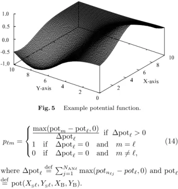
The following potential function is presented for reducing the control space and solving this problem.
pot(X, Y, XB, YB) = exp(−c((X−XD)
2+ (Y −Y
D)
2))
− exp(−c((X−XB)2+ (Y −YB)2)), (13)
where c is a constant (set to 0.1 here) and (XB, YB)
is the coordinate that gives the minimum value of the potential function. The potential function for (XB, YB) = (1.0, 8.0) and (XD, YD) = (5.0, 0.0) is shown in Fig. 5 as an example. Routing probability p`m for
m ∈ {`, n`1, n`2, · · ·,n`NAN`} is given by
Fig. 5 Example potential function.
p`m= max(potm− pot`, 0) ∆pot` if ∆pot`> 0 1 if ∆pot`= 0 and m = ` 0 if ∆pot`= 0 and m 6= `, (14)
where ∆pot`def= PNAN`
j=1 max(potn`j− pot`, 0) and pot` def
= pot(XS`, YS`, XB, YB).
The potential function denotes relative routing probabilities. This means that packets are transmitted from a node with a lower potential to one with a higher potential. On the basis of the potential function in Eq. (5), the routing probabilities p`mfor all nodes are
deter-mined by setting only two variables (XB, YB). Thus,
by applying Eqs. (13) and (14) to routing problems and setting control input u to (XB, YB)t, we can reduce the
dimension of the control space fromPNSN
`=1 NAN`to 2.
3.3 Nonlinear Approach to Robust Routing
Consider a time-invariant environment in which λ`;tfor
∀` is a constant. In this environment, q`;t and e`;t
con-verge to constants if the routing probabilities are fixed. Thus, the routing problem is reduced to the problem of maximizing limt→∞rt with respect to the routing
matrix: max
P t→∞lim rt, (15)
where P is the NSN × (NSN+ 1)-routing matrix with
elements p`m.
Next let us consider an environment in which the
λ`;t vary with time. Let xt be a state variable
com-prised of some or all of λ`;t, q`;t, and e`;t, and let the
routing matrix be the control input. The dynamic rout-ing problem is thus reduced to a nonlinear control prob-lem: ( max Pt Rt xt+1= fnet(xt, Pt), (16) where Rtis the discount return defined by Eq. (2), Pt
environment.
The dimension of the control space in Eqs. (15) and (16) is PNSN
`=1 NAN`, which is too large to obtain
the optimum route, as mentioned above. By applying Eq. (14) to Eqs. (15) and (16) and setting control input
u to (XB, YB)t, we obtain the following equations:
max u t→∞lim rt, (17) ( max ut Rt xt+1= fnet(xt, ut). (18) Using these equations, we can search for the opti-mum route in the two-dimensional control space. Al-though the dimension of the state space in these equa-tions remains high, we can use the actor-critic method with RWPCA and AIA, which works well in a high-dimensional state space, to solve them. The perfor-mance of the routing algorithms with the potential model and the actor-critic method with RWPCA and AIA is presented in the next section.
4. Performance Evaluation
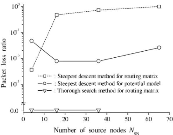
4.1 Static Routing for Time-Invariant Environment Three routing strategies for a time-invariant environ-ment were examined using the network model described in Sect. 3.1 to evaluate the effect of the potential model presented in Sect. 3.2.
• Steepest descent method for routing matrix: In a
time-invariant environment, it is not necessary to use reinforcement learning because the problem can be solved, as shown in Eq. (15), by searching for the value of the routing matrix that provides the max-imum value of limt→∞rt. Thus, a simple nonlinear
programming technique can be applied to the prob-lem. In this paper, the steepest descent method is used because it is used in the actor-critic method to update ξdi and ηdi in Eqs. (2) and (3).
• Steepest descent method for potential model:
Equa-tion(17), which is based on the potential model scribed in Sect. 3.2, is solved using the steepest de-scent method.
• Thorough search method for routing matrix: For p`m
∈ {0, 1}, the optimum solution for Eq. (15) is
ob-tained by conducting a thorough search for all com-binations of p`m.
Let λalldef=
PNSN
`=1 λ`be the total packet generation
rate and λ` be constant. Set λ` of the source nodes in
S1 and S4 to 1.9 × λall/NSN, λ` of the source nodes
in S2 and S3 to 0.1 × λall/NSN, λall to 3.6, C to 2,
and b to 32. If p`m are appropriately determined, it
is clear that most packets generated at the nodes in S1 are transmitted through S2 and S3 and that the
packets generated at the nodes in S4 are transmitted
to the destination node without passing through other
Fig. 6 Effect of potential model on static routing. regions. It is also clear that all packets arrive at the destination node without any loss becausePNSN
`=1 λ` =
λall= 3.6 ≤ 2C.
The packet loss ratios obtained using the three strategies for a time-invariant environment are shown in Fig. 6. The thorough search method provided the op-timum solution although it worked only for NSN ≤ 36
because of the calculation cost. The steepest descent method for the routing matrix worked well (i.e., the packet loss ratio was sufficiently small) for NSN = 4,
but the solutions for NSN≥ 16 were not optimum. This
is because the dimension of the control space is too high when NSN is large, so the method causes routing loops
and falls to a local optimum. While the packet loss ratio of the steepest descent method for the potential model was not optimum for NSN = 4, those for NSN ≥ 16
were sufficiently small. This is because the dimension of its solution control space remains two independent of
NSN. Thus, the potential model is effective for solving
the routing problem except when NSN is small.
4.2 Dynamic Routing for Time-Varying Environment Consider a time-varying environment in which two re-gions are randomly selected from S1, S2, S3, and S4
at periodic intervals of Tλ. The λ`;t of the nodes
in the selected regions are set to 1.9 × λall/NSN, the
λ`;t of the nodes in the other two regions are set to
0.1 × λall/NSN, λall is set to 3.6, C to 2, b to 32, and
Tλ to 100. Although λ`;t varies at intervals of Tλ, Pt
can be determined without any packet loss because PNSN
`=1 λ`;t = λall = 3.6 ≤ 2C in the same manner as
in the time-invariant environment. To evaluate the ro-bustness of routing algorithms, a disturbance noise was introduced at a node adjacent to the destination node. The noise was a random variable from 0 to buffer length
b and changed with period Tnoise. It prevented the other
nodes from observing the queue length of the adjacent node.
Because the potential model is effective, as shown in Sect. 4.1, the effect of RWPCA and that of AIA were evaluated using the following three routing
strate-Fig. 7 Effect of RWPCA and AIA on packet loss ratio (NSN=
16, Tnoise= 8).
gies based on the actor-critic method. They observe
xtdef= (λ1;t, q1;t, · · · , λNSN;t, qNSN;t)
t, and routing
prob-lems are solved using Eq. (18), which is based on the potential model. Routing matrix Pt is determined by
Eq. (14). Q-routing [5] was also evaluated to isolate the effect of RWPCA and AIA.
• Actor-critic method with RWPCA and AIA: As
sho-wn in Sect. 2.4, RWPCA transforms xt to st
us-ing Eq. (7) and basis {φi(s)} is constructed by AIA.
Control input u is determined using the actor-critic method.
• Actor-critic method with RWPCA [8]: This strategy
does not use AIA. Basis {φi(s)} is constructed on
the basis of Dk given by the Cartesian product as
Dk = Dk1× Dk2×, · · · , ×Dkds, and Nd is determined on the basis of the standard deviation in st.
• Actor-critic method with AIA [9]: This strategy does
not use RWPCA and thus sets xtto st.
• Q-routing: Q-routing [5] is the most well-known
rout-ing method based on reinforcement learnrout-ing. It as-signs a Q-value to each adjacent node on the basis of learning [4] and selects the route using the Q-value. The Q-value of each node is updated with step size ζQ on the basis of the queue length of the adjacent nodes.
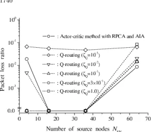
The three routing algorithms based on the actor-critic method were evaluated for NSN= 16, Tnoise= 8,
and various values of N in an environment with distur-bance noise. As shown in Fig. 7, the packet loss ratios obtained were sufficiently small when N was 256, and those obtained by the actor-critic method with RW-PCA and AIA were the smallest except when N was 16. These results show that the adverse effect of dis-turbance noise can be effectively eliminated by using both RWPCA and AIA except when N = 16 compared with using only RWPCA or AIA. This is because the states of all the nodes are taken into account, RWPCA and AIA complement each other, and they work con-sistently by taking the immediate reward into account. In an environment with disturbance noise, the packet loss ratio was evaluated for NSN= 16, N = 256,
Fig. 8 Effect of disturbance noise on packet loss ratio (NSN=
16, N = 256).
Fig. 9 Effect of disturbance noise on packet loss ratio for dif-ferent traffic pattern (NSN= 16, N = 256).
and various values of Tnoise to investigate the
robust-ness of Q-routing and the effectiverobust-ness of the actor-critic method with RWPCA and AIA. Figure 8 shows that the packet loss ratios obtained by the actor-critic method with RWPCA and AIA were sufficiently small regardless of Tnoise although the packet loss ratios of
Q-routing increased as Tnoise increased. Figure 9 shows
the packet loss ratios evaluated for a traffic pattern different than that used for Fig. 8: NSN/2 source
nodes were randomly selected, their λ`;t were set to
1.9 × λall/NSN, and the λ`;t of the other source nodes
were set to 0.1 × λall/NSN. Figure 9 shows that the
actor-critic method with RWPCA and AIA was robust in the same manner as in Fig. 8. The reason Q-routing was affected by the disturbance noise is that Q-routing directly uses the queue length, which was disturbed by the noise. In contrast, the actor-critic method with RWPCA and AIA eliminates the effect of noise from the state by using RWPCA and AIA. We can thus con-clude that the actor-critic method with RWPCA and AIA is robust and able to cope with various traffic pat-terns.
Figure 10 shows the packet loss ratio for N = 256 and various values of NSNwhen a disturbance noise was
Fig. 10 Effect of number of source nodes on packet loss ratio (N = 256).
small when 16 ≤ NSN ≤ 36 except for Q-routing with
ζQ = 10
−3. However, when N
SN was large, the packet
loss ratios of both algorithms were higher; that is, it is difficult to keep the packet loss ratio small when NSN
is large, apparently because the packets are stored in more nodes when NSNis large, making it more difficult
to control them. Although the packet loss ratio can be reduced by increasing buffer length b of each node, this is problematic because it causes a longer delay time.
The potential function in Eq. (13) is very simple and has only one maximum value and one minimum value. This is because it was made for a network that has only one destination node and packet traffic that is not complicated. Thus, it cannot express the compli-cated packet traffic that arises in a network when NSN
is large. This problem could be solved by improving the potential function, which remains for a future study. 5. Conclusion
Routing problems were formulated as nonlinear con-trol problems, and the high-dimensional concon-trol space of the problem was reduced to a two-dimensional con-trol space by using newly developed concon-trol space com-pression based on a potential model. The state space of the problem was compressed using reward-weighted principal component analysis, and a basis for approx-imating a control function was adaptively constructed using activity-oriented index allocation. A routing al-gorithm based on these methods and the actor-critic method can efficiently search for an approximate opti-mum route even if the routing information is disturbed. References
[1] C. Karlof and D. Wagner, “Secure routing in wireless sen-sor networks: Attacks and countermeasures,” Ad Hoc Net-works Journal, vol. 1, pp. 293–315, Sept. 2003.
[2] J. Broch, D. A. Maltz, D. B. Johnson, Y. C. Hu, and J. Jetcheva, “A performance comparison of multi-hop wire-less ad hoc network routing protocols,” Proc. 4th Annual ACM/IEEE International Conference on Mobile
Comput-ing and NetworkComput-ing, pp. 85–97, 1998.
[3] C. Huitema, Routing in the Internet, Prentice Hall, USA, 1995.
[4] R. S. Sutton and A. G. Barto, Reinforcement Learning, MIT Press, USA, 1998.
[5] J. A. Boyan and M. L. Littman, “Packet routing in dy-namically changing networks: a reinforcement learning ap-proach,” Advances in Neural Information Processing Sys-tems, vol. 6, pp. 671–678, 1993.
[6] S. Kumar and R. Miikkulainen, “Confidence based dual re-inforcement Q-routing: an adaptive on-line routing algo-rithm,” Proc. 16th International Joint Conference on Arti-ficial Intelligence, pp. 231–238, 1999.
[7] Y. Zhang, J. Liu, and F. Zhao, “Information-directed rout-ing in sensor networks usrout-ing real-time reinforcement learn-ing,” Combinatorial Optimization in Communication Net-works, Chapter 10, Springer, pp. 259-288, 2006.
[8] H. Satoh, “A state space compression method based on multivariate analysis for reinforcement learning in high-dimensional continuous state spaces,” IEICE Trans. Fun-damentals, vol. E89-A, no. 8, pp. 2181–2191, Aug. 2006. [9] H. Satoh, “Feature space construction and function
ap-proximation for reinforcement learning,” Tech. Rept. IEICE NLP2006-41, pp. 43–48, July 2006.
[10] R. A. Johnson and D. W. Wichern, Applied Multivariate Statistical Analysis, 5th ed, Pearson Education, Prentice Hall, USA, 2001.
[11] I. Menache, S. Mannor, and N.Shimkin, “Basis function adaptation in temporal difference reinforcement learning,” Annals of Operations Research, vol. 134, no. 1, pp. 215–238, Feb. 2005.
[12] H. Satoh, “Reinforcement learning for continuous stochastic actions – An approximation of probability density function by orthogonal wave function expansion –,” IEICE Trans. Fundamentals, vol. E89-A, no. 8, pp. 2173–2180, Aug. 2006. [13] K. Doya, “Complementary roles of basal ganglia and cere-bellum in learning and motor control,” Current Opinion in Neurobiology, vol. 10, no. 6, pp. 732–739, Dec. 2000.