Variation of water table fluctuation in paddy fields shown by coefficient of variance (II)-香川大学学術情報リポジトリ

Vol 21 (No.48) (1970) 139

VARIATION OF WATER TABLE FLUCTUATION

IN PADDY FIELDS

SHOWN

BY

COEFFICIENT OF VARIANCE

Kiyoshi

FUKUDA,

Katsuhi ko

I z u ~ s u ,

Tadao MAEKA

W A

1.

Introduction

In the previous paper's, the variations of the fluctuation in the region during an annual cycle were estimated more generally by using a stochastic method.

This time, in this paper, we have tried to show the degree of the fluctuation of the water table in the paddy fields during a given month for a well by using the coefficient of variance of the water table depth measured daily.

This paper is the sequel to the paper having the same title, and also the 17th report of "Shallow Ground Water in the Downstream Basin of the Aya River."

2. Theoretical Procedure

In order to show the degree of the fluctuation of the water table in paddy fields for a given month for a well, the coefficient of variance(I), C, was used.

If D is defined a s the depth of the water table measured from the ground surface of a well for a day, the degree of the fluctuation of D for a well for a given month can be calculated by using Eq. (1).

where D=magnitude of D for a day,

M= arithmetic mean,

n=number of terms in the series.

The average values of C for a particular month during m annual cycles can be calculated by Eq. (2)

where Ci=the magnitude of C for a well for z, the month of an annual cycle, m=number of months of the annual cycles.

In this case, the data for D was taken from the daily field observations the four annual cycles (from March 1965 to February 1969) ; therefore the values of m were given as 4.

140 Tech. Bull,, Fac. Agr. Kagawa Univ..

From Eq. (1)

,

Eq. (3) was obtained.

Thus, the values of M-t d and M-d can be calculated. For the particular. months, the

_-

values of M t d and M-d can also be calculated and these are expressed as D Z + ~ and

~ z - a .

3.

Results and Discussion

3.1

Variation of during the annual cycle

-

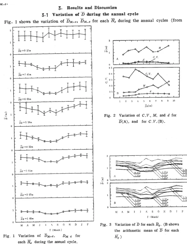
Fig. 1 shows the variation of &+,z, Da2-d for

F i g . =2 5701

1

1

ij6 = I 65m 0 M A M l l Z S O U D J F T (Month )

1 Vaxiation of & + d , Dx d for

each

BD

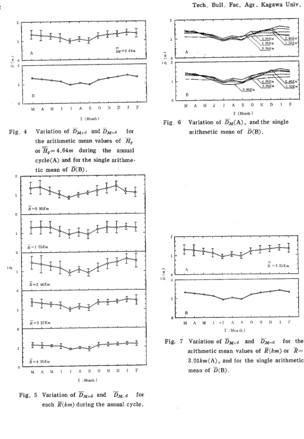
during the annual cycles (from

Fig 2 Variation of C. V , M, and d for

-

D ( A ) , and for C V.(B).

F!g. 3 Variation of D for each

Bg

(B shows the arithmetic mean of fox each

-

Hg 1

Vo1.21 (No. 48) (1970) 141

March to February). By Visual-observation of Fig: 1, i t is seen that there are depressions of the values of

Dz+~

3%-a

during the irrigation period (from June to September) except in the case of

H,

=9.27m (the upper graph of Fig. 1) .And also it seems that the larger the values of H,, the larger the degree of the depression except in the case of H, =9.27m.

-.

In order to see the degree of the fluctuation of D&+<,

D M

during the annual cycle for each I%, the values of the coefficient of

fix

(C. V.) were calculated as shown in Fig. 2A.

The values of C. V. of D (the solid line) varied from 0.067

(H,

=9.27m) to 0.224

(f7Q

=4.22m) ; the values of the standard deviation of D(the dotted line) varied from 0 . 0 9 6 ~ ~ (zg=2.57m) to 0 . 2 6 ~ ~ <'H9=4.22m); and the values of the mean of D (&) (the dot-dashed line) varied from 0.821 m (Hg=1.65m) to l.44m(Hg=5.58m).

As shown in Fig. 3A, the curves (showing the time series of

D)

seem to converge into two groups during the period from July, August, and September. These two groups are: 1) the upper group of curves having D for Hg=2.57m, 3.64m, 5.58m, and 6 . 6 1 ~ ~ ; and 2) the lower group having D for H ~ = 1.65m, 4.22m, and 7.41m. It is thought that the curve of D for Hg= 9.27m is an exception.

For each group of curves, i t is seen that the curves roughly over-lap each other in the three particular months. In another words, the values of for each

Hi

in both groups (the upper or lower) seem to converge into constant values respectively during the three particular months.

During the irrigation season, the paddy fields are full of irrigation water, thus, the water table of shallow groundwater in paddy fields rises. Most of the study area was occupied by the area having D=O.O m to 1.0 m (the shallowest water table during an annual cycle) as shown in the previous paper(2).

The factors mentioned above are one of the reasons why the values of

D

for each month on each curve in Fig. 3A converge into constant values during the three particular months.

From the figure for the upper group of curves the constant values are read as follows: 0.89m in July, 0.90m in August, and 0 . 8 9 ~ in September, and (for the lower group), 0 . 7 1 ~ ~ in August, and - 0 . 7 3 ~ ~ in September.

In order to confirm the values of

D

for each

pg,

the arithmetic means of D for each

g,

were calculated, and the results of the calculation are shown in Fig. 3B. The values of in Figs. 3A and 3B are much the same.

Fig. 4A shows the variation of D M , & and for the arithmetic mean values of

p,

(these varied from Hg = 1 . 6 4 ~ ~ to H, =9.27m) or cHg) =4.64m during the annual cycle.

In order to confirm the variation of the values of during the annual cycle, the arithmetic mean of D was calculated as shown in Fig. 4B. The values of the time series of D in Fig. 3B and the one of

Ba

are much the same.

The curves in Figs. 4A and 4B and the ones in Figs. 7A and 7B lie one above the other. Therefore, the values of

D

or

3 , ~

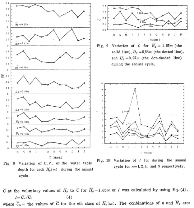
in these figure are much the same.

Fig. 5 shows the time series of

D Z + ~

and D & - b for each R(km) during the annual cycle. The values of

Bx+d,

and DZ-a for each

R

make the curves depression during the

Tech,, Bull,, Fac. Agr

.

Kagawa Univ.

T ( M o n t h )

Fig 4 Variation of fix+r~ and &-# for

t h e arithmetic mean values of -FI,

or

zg

= 4 . 6 4 ~ during the annual cycle(A) and for t h e single arithme. t i c mean of p(B).

2 , . . . . - 1

M A M J I A S O N D I F

I (Month

Fig. 6 Variation of D=(A) , and the single arithmetic mean of D(B).

-.

Fig. 7 Variation of D ~ , R and DH-d for the arithmetic mean values of z(1zm) or %'-- 3 Olkm(A), and for the single arithmetic mean of D(B)

.-

Fig. 5 Variation of p x + d and D X - d for each R ( k m ) during the annual cycle.

Vo1 .21 (No. 48) (1970) 143

irrigation period (from June to September). And the degree of the depressions seems to vary with the values of h?.

In order to see this degree, the coefficient of the variance of

5

was calculated. The values of C. V. of D(the solid line) varied from 0.091

( K

=4.35/~m) to 0.184(11= 2.46km). The values of the standard deviation of D varied from 0.098nz (K-4.35km) to 0.234m<~=2.46km). And the values of the mean of D varied from 1 . 0 7 8 ~ ~ (X=4.35knz) to 1.289m ( ~ = 3 . 2 7 k m ) .

As shown in Fig. 6A, the curves of D;CL are roughly one above the other during the period of the irrigation months (from June to September).

This means that the water table of most of the study area is 0 . 9 2 ~ ~ in July, 1.04nz in August, and 0.98m in September, respectively.

The arithmetic mean of

IS

was calculated in order to confirm the variation of D during the annual cycle, and the result is shown in Fig. 6B. The curves in Fig. 6B and Fig. 6A are much the same.

From Fig. 6A, the values of D.X in July, August, and September are found to be

0.92m, 1.00m, and 0.91m, respectively. These values of D ll are much the same as the

ones in the upper group of the curves in Fig. 3A.

Fig. 7A shows the time series of

EN,,,

and for the arithmetic mean values of R

(varying from 0.96km to 4.35km) or

( E )

-3.01km during the annual cyc:e. Fig. 7B shows the time series of D that was obtained by the single alithmetic mean method. And the values of

D X

in Fig. 7A and D in Fig. 7B are much the same.

3.2 Variation of C during a n annual cycle

In order to see how the water table of shallow groundwater in the paddy fields fluctuates during the annual cycle, the term C. V. was used. If the time series of C. V. of the water table depth,

E,

for each month is made for each

H,,

the fluctuation of D can be estimated by C. V. of D.

Fig. 8 shows the variation of C. V. of the water table depth for each

n,

during the annual cycle.

In order to evaluate the degree of the fluctuation of the values of

C

during the annual cycle for each

a,

the values of the coefficient of variance (C.V.), the standard deviation, and the mean of

C.

V. were calculated as shown in Fig. 2B.

The values of the coefficient of variance varied from 0.202 (H9=9.27m) to 0.475 ( H ,

- 3.64m). The values of the standard deviation varied from 0.032 ( H g = 1.65m) to 0.064

(g,

=6.61m). And the values of the mean of

C

varied from 0.085(HV=1 .65nz) to 0.267

(z,=

9.27~2).

As shown in Fig. 9, the curve of C for H, =9.27m runs above the curve of

-d for

H,=

5.58% and the curve of

C

for H,=5.58m runs above the curve of C for H ,=1.65nz throu- ghout the annual cycle. Therefore, it seems that the larger the values of H, the greater the values of C.

144 Tech, Bull. Fac. Agr

.

Kagawa Univ. 0 4 0 3 10 0 2 0 1 0 0 M A M I J I I O N D J F 1 (Month )

Fig. 9 Variation of C for = 1 65m (the solid line), H, =5.58m (the dotted line), and H; =9.27m (the dct-dashed line) dux ing the annual cycle.

I (Month)

Fig. 10 Variation of I for during the annual Fig 8 Variation of C V. of the water table

cycle for n = 1 , 2 , 4 , and 9 rcspectively depth for each Ii,(m) during the annual

cycle

--

C at the voluntary values of H, to ? for Hg = 1 . 6 5 ~ or I was calculated by using E q . ( 4 ) .

I=

C/Tz

( 4 )

where

z,

= the values of C for the nth class of s ( m ) . The conbinations of n and I-& are: (n= 1 , H , = 1.65m), (2,2.57m), (3,3.64m)

,

( 4 , 4 . 2 2 ~ ~ ) ~ ( 5 , 5.58m), ( 6 , 6 . 6 1 ~ ) ~ (7, 7 . 4 1 ~ ) ~ and ( 9 , 9 . 2 7 ~ ~ ) . The values of H~ that paired with n=8 were zero because there were no wells having their height between 8 . 0 0 ~ and 9.00m or 8 . 0 0 ~ S H g 1 9 . OOWZ.

= the values of (: for class- 1 or for Hg = 1.65m. The results calculated by Eq.(4) are shown in Fig. 10.

As shown in Fig. 10, the larger the values of n in Eq. (4), the larger the values of I. The maximum values of I during the annual cycle for each n varied from 1.8 ( n = 2 , or Hg=2.57m) to 9,15 (n=9, or &=9,27m); the minimum values of I varied from 0.41(n=2 and 3 , or H,=2.57m and 3 . 6 4 ~ ~ ) to 1 93 ( n = 9 ) ; and the mean values varied from 1.17

Vo1.21 (No .48) (1970) 145

Fig. 11 Time series of (the arithmetic mean of C for all the

&

(m)) for the annual cycle.

Fig. 11 shows the time series of

z,

(the arithmetic mean of

C

for all the

&)

for the annual cycle. The values of

c

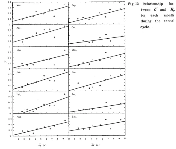
varied from 0.10 (January) to 0.23 (April).

Fig Relationship be-

. --

tween and H,

for each month during the annual cycle.

Fig. 12 shows the relationship between C and Hi for each month during the annual cycle. From the data plotted in these graphs, the linear equation Eq. (5) showing the relation of

C

and .H, was obtained by using the least square method.

145 T e c h Bull. Fac Agr Kagawa Univ

The second term was divide3 by H,I (H,=lm) in order to give a dirrensionless variable to this term.

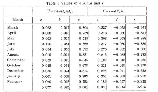
Table I Values of a , b , c , d and r

The values of b, a , and r(tbe correlation coefficient betwee2 C and-&) for each month

-

C ~ a i bHg/Hol

I

c = c - ~ & R , I

- - - -- - - - --- - - - -

I

. -

I

Month I b r I

-

I n

I

are listed in the left side columns of Table 1.

These values varied as the month went on, and, the values of r varied from 0.661

o

8021

o

337l -0 052i -0 971

March April

(February) to 0.. 892 (July). The mean was 0.790. Therefore these equations (the solid

o

053'

o

027

lines in Fig. 12)roughly express the relationship between (: arid H,.

I

---I

From these equations it can be said that the higher the height of the well sites, the greater the values of for each month throughout t'ne annual cycle In other words, the

May Juce J U ~ Y August September October December

higher the height of the well sites, the greater the fluctuation of the water table.

Fig. 13 shows the relationship between c a n d

i?

for each month throughout the annual 0 0081 0 028 0 01.2 0 02: -0 100 0 081 -0 0541

'

0 0024 O Olol 0 02.1 0391 0 014 0024

cycle. From this data (the open circles in Fig. 13), the linear equation showing the C - R

relationship, Eq (6), was obtained by using the least square method.

-0 811 -0 988 -0 889 0 880 -0793 -0 235 -0.779 - 0 6 8 2 0 769 0 373 -0 0:O 0 i 2 5

o

303 0 058 0 862 0 377 -0 060 0 3 5 0 892 0 276 0 052

In order to give the dimensionless variable for both sides of the equation, the second -0 910 -0 830 -0.915 - - -- - 0.881 0 845 0 678 0-814 January 0 793 February 0 752 0 661 .- - -- - - - - -

-term on the right hand side of Eq (6) was divided by 121 (R=llzm).

The values of c , d , and r are listed in the right hand columns of Table 1. 0 2 1 6 -0032

0 1891 -0 013 0 211 - 0 02: 0298' - 0 0 4 1

The values of Y varied from -0.235 (September) to -0.988(May) and the mean was

0 308 0 184 0 310

- - --

-0..807. Most of the values of r., however, are over - 0.682. Therefore i t is thought that -0 060

-0 027

- 0 044

- - - -

the value r = -0.235 is an exception and the equation is therefore sufficient t o practically express the relationship between and

2 .

The solid line in Fig. 13 shows the equation for each month.

Vo1 , 2 1 (No

..

48) (1970) 04 0 3 0 2 01 0 03 0 2 J u l - Jan - . Eeb .

From these graphs, i t is seen that the larger the values of the smaller the val- ues of C. In other words, the-nearer to the sea coast the study area, the smaller the degree of fluctuation of the water table.

4.

Summary

1) The degree of the fluctuation of the water table in the paddy fields during a given month for a well was calculated by using the coefficient of variance (C) of the water table depth (D) of each well. By this, the variance of D during the annual cycle

(March to February) was obtained.

2) The relationship between C and H,

(the height of well sites) for each month was expressed as Eq. (5). The mean value of r (coefficient of correlation) was 0.79.

The relationship between C and R (the distance in km of the well sites from the fan- head) for each month was expressed as

Eq. ( 6 ) . The mean value of Y was - 0.81

.

5.

Acknowledgements

0 1

The writers wish to thank Mr. Yoshi-

01

kazu KUSANAGI, a graduate student a t Ka-

0

0 1 2 3 4 5 1 2 3 1 5 gawa University, and Mr. Takashi OSAKA,

n

( K r n ) an undergraduate student at the same Uni

-

R

( K m )

versity, for their help in carrying out this Fig. 13 Relationship between C and-R for each _{investigation.}

month t h ~ oughout the annual cycle

.

A part of the expenditure was defrayed by a research grant from the Ministry of Education.

References

(1) C H E B O T A R E V , N . P . : Theory of Stream Runoff (translated from Russian), I.srae1 Program ,for.

Scient<ftc Translations, ,Jerusalem, 18-24, (1966).

(2) FUKUDA.K.. : Tech.. Bull. Fac. A g r . Kagawa Univ., 18 208-229, (1967).

148 Tech. Bull. Fac,, Agr, Kagawa Univ.,

7kfflJ&@~%Ei&T7kii~ D &

6 A

H @$ag4ED%$iEaab@B%B%3% L , Z h K A 9 T%DA Dt&T7k@ 0

g B @ % S b L k . $ k , C h 6 D (A P ~ D ) ~ ~ k @ D ~ B d K a d K 6 @ % ? U B % k .

i&T7ki$@@U (C) D@wiJ#lDl& (Hg(m)) 2DWi%M,

&a

2 %Eq. (5)Dd: 3 Kg#$ (T%D~€IWl%BT=

0.79) - c % $ h k 5 k , C ~ B B ~ # D B J B ~ ~ L bDFE%(R(km)) 2 0>N4%%, &A 2 %Es 16)Dd: 3 K, AGJEDB j&(r=o.sl)

-c$sha27"c.

k & , z D@%KZL~RHD-%BL;X,

A%V$kiH%%RB

(@X@%. 7k-i(Y. H I ) Vc k 9 T 3 t L 5 C

$k Z

z

K12L

-c,

% ~ % S ; h ? .