Title
Observation of νμ→νe oscillation in the T2K experiment(
Dissertation_全文 )
Author(s)
Ieki, Kei
Citation
Kyoto University (京都大学)
Issue Date
2014-03-24
URL
http://dx.doi.org/10.14989/doctor.k18063
Right
Type
Thesis or Dissertation
Observation of ν
µ→ ν
eoscillation in the T2K
experiment
Kei Ieki
February, 2014
Department of Physics, Graduate School of Science
Kyoto University
Observation of ν
µ→ ν
eoscillation in the T2K
experiment
A dissertation
submitted in partial fulfillment of the requirements
for the Degree of Doctor of Science
in the Graduate School of Science, Kyoto University
Kei Ieki
Department of Physics, Graduate School of Science
Kyoto University
Dissertation Committee: Tsuyoshi Nakaya Atsuko K. Ichikawa Koji Tsumura Masayuki Niyama Takeshi Go Tsuru
Abstract
The T2K experiment is an accelerator based long baseline neutrino oscillation experiment.
The νµ beam is produced at J-PARC in Tokai, and detected 295 km away from the production
target by the Super-Kamiokande (SK) detector. In this thesis, we present the νµ→ νeoscillation
measurement from the T2K experiment that clearly demonstrates, at the 7.3σ significance,
evidence for νe appearance. The measurement of νµ→ νe oscillations is of a particular interest
because this mode is sensitive to both mixing angle θ13and CP phase δCP of the mixing matrix.
Precision measurement of νµ→ νeallows to explore the CP violation in the lepton sector, which
is yet to be observed.
The identification of neutrino interaction modes is important in the measurement. In T2K,
we select CCQE interaction (ν + n→ l + p) as a signal, while the main background for CCQE
is CC1π interaction (ν + N → l + N′+ π). A full-active fine-grained detector (FGD) is capable
of identifying the interaction modes by detecting the short pion tracks in the final state. The interaction of pions with nuclei significantly affects the identification of neutrino in-teraction modes. For example, when the pion absorbed by a nucleus before being detected, CC1π interaction is misidentified as CCQE interaction. The uncertainty of the pion-nucleus
interaction is one of the dominant systematic error sources in the T2K νµ → νe measurement.
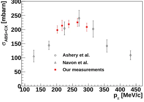
We performed a pion-nucleus interaction measurement at the TRIUMF pion beamline, using a finely-segmented scintillator fiber detector. The sum of pion absorption and charge exchange
interaction cross sections on carbon is measured with uncertainty of ∼6.5%, which is roughly
half of the error of the past experiments. Using our new data set together with other external data sets, we improved the pion-nucleus interaction model used in T2K. The uncertainty of the
pion-nucleus interaction was reduced to∼1/4. The improved model is not used in the oscillation
analysis yet, but the pion-nucleus uncertainty will become negligible in the future once we use the improved model.
The main topic of this thesis is the measurement of νµ → νe oscillation. There are 28 νe
candidate events observed at SK, with the T2K beam data collected from Jan. 2010 to May. 2013
(corresponding to 6.57×10²⁰protons on target). Using the momentum and angular distribution
of the outgoing electrons observed at SK, we performed a maximum likelihood fit to measure the
oscillation parameters. Assuming δCP= 0 and normal (inverted) hierarchy, we obtain a best fit
value of sin22θ13= 0.136+0.044−0.033(0.166−0.042+0.051). In the fit, the uncertainty of sin2θ23and ∆m232 are
taken into account using the constraints from T2K published νµ disappearance measurement.
The significance to exclude θ13= 0 is 7.3σ. This is the first measurement to discover the νµ→ νe
with more than 5σ. Furthermore, this is the first discovery of the appearance of different neutrino flavour from neutrinos of another flavour with >5σ significance. We obtain the 90% exclusion
region for δCP by combining the T2K result with the world average value of θ13 from reactor
experiments.
Normal hierarchy: 0.604 ∼ 2.509
Inverted hierarchy: −3.142 ∼ −3.043, −0.132 ∼ 3.142
Although the constraint on δCP is still weak to claim a discovery of non-zero δCP, this result is
Acknowledgements
For the six years of my life as a graduate student, I was extremely lucky to have supports of many people. Without their help, I could not realize this thesis.
First of all, I would like to express my gratitude to Tsuyoshi Nakaya, for always leading me to the right way. He also gave me a lot of opportunities to have precious experiences. His advice and attitude made me rethink my own stance and attitude as a researcher. I also want to express my thanks to Atsuko Ichikawa. She gave me a lot of advices at the meeting, which were often very crucial and productive. I also want to express my gratitude to Akihiro Minamino who gave me a lot of advice for my analysis.
I would like to give special thanks to the member of the DUET experiment. I owe a big thanks to Motoyasu Ikeda, who helped me not only in the research but also in the private life. I would like to thank him for his patience over the years supporting me and leading the DUET experiment. I would like to thank Takahiro Yamauchi for being a core member of PIAνO team. I owe a great deal of thanks to Hirohisa A Tanaka and Michael Wilking, who helped me not only as the DUET collaborators, but also as the member of the FGD group. I would like to give many thanks to Kendall Mann, for supporting me in DUET, in the oscillation analysis and in the life in Vancouver. I am also grateful to everyone who helped me in the DUET experiment including Masashi Yokoyama, Yoshinari Hayato, Yasutaka Kanazawa, Patrick de Perio, Elder Pinzon, Sampa Bhadra, Charles Cao and Matt Gottshalk.
My work in T2K started in 2008. Especially in the first two years, I spent a lot of time working with people from Canadian group. I am really glad to have been able to work with
them. I would like to thank Scott Oser, Thomas Lindner, Fabrice Retiere, Akira Konaka,
Nicholas Hastings, Daniel Brook Roberge, Caio Licciardi, Brian Kirby, Shimpei Tobayama, Jiae Kim and all other people who worked with me. I never forget the taste of Hitachi beef which we had at the collaboration meeting in 2014. I hope to have chance to work with you again in the future.
I owe a huge thanks to Christophe Bronner and Ken Sakashita, who worked with me for the oscillation analysis. I learned a lot from the discussion with them, and it was my honour and great pleasure to work with such bright and talented people. I would like to also thank Yasuhiro
Nishimura and Joshua Hignight for the discussion of the νe analysis results. My work on the
oscillation analysis is directly dependent upon the hard work of the oscillation analysis group. I want to express my gratitude to all the T2K members and people in the J-PARC, KEK and SK group.
Living in Tokai with T2K collaborators was really fun. I would like to thank Akira Murakami, Kento Suzuki, Shota Takahashi, Tatsuya Kikawa and Kunxian Huang staying at Ohta-danchi with me. It was nice to have Nabe party with sake and games with you. I enjoyed both physics discussion and meaningless discussions. I wish to extend my thanks to Masashi Otani, Hajime Kubo, Kodai Matsuoka, Takatomi Yano, Takahiro Hiraki, Seiko Hirota, Megan Friend, Ryoske Ohta and Phillip Litchfield.
Kyoto University is the place I’ve spent most of the time in the last years. I must thank all the other members in our laboratory: Masaya Ishino, Tadashi Nomura, Hajime Nanjo, Toshi
Sumida, Saki Yamashita, Naoki Kawasaki, Takahiko Masuda, Daichi Naito, Yosuke Maeda, Shigeto Seki, Takuya Tashiro, Tokio Nagasaki, Shinichi Akiyama, Naoyuki Kamo, Keiji Tateishi, Takaki Hineno, Yuuki Ishiyama, Ichinori Kamiji, Takuto Kunigo, Jiang Miao, Kota Nakagiri, Keigo Nakamura, Tatsuya Hayashino and Kento Yoshida.
I would like to acknowledge supports from the Japan Society for Promotion of Science (JSPS) and the global COE program.
Finally, I would like to send my best thanks to my family.
Kei Ieki Kyoto, Japan February, 2014
Contents
I Neutrino oscillation 1
1 Introduction 2
1.1 Neutrino oscillation . . . 2
1.1.1 Three flavours of neutrinos . . . 2
1.1.2 Discovery of neutrino oscillation . . . 3
1.1.3 Theory of neutrino oscillation . . . 3
1.2 Current knowledge of neutrino physics . . . 6
1.2.1 Oscillation parameters . . . 6
1.2.2 Unanswered questions . . . 8
1.3 Motivation of νµ→ νe measurement . . . 11
1.4 Outline of this thesis . . . 12
II T2K experiment 14 2 Overview of the T2K experiment 15 2.1 J-PARC neutrino beam line . . . 16
2.1.1 Controlling the primary proton beam . . . 16
2.1.2 Off-Axis method . . . 18
2.2 Monitoring of the secondary beam . . . 19
2.2.1 Muon monitor . . . 21
2.2.2 INGRID . . . 21
2.3 ND280 and Super-Kamiokande . . . 22
2.3.1 Neutrino detection at ND280 and SK . . . 22
2.3.2 ND280 . . . 23
2.3.3 Far detector (Super-Kamiokande) . . . 25
2.4 Summary of the beam data taking . . . 25
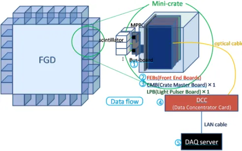
3 The Fine-Grained Detector 28 3.1 FGD and neutrino interaction . . . 28
3.2 Fine-Grained Detector . . . 29
3.2.1 Overview of the design . . . 29
3.2.2 Readout electronics . . . 30
3.2.3 MPPC (Multi-Pixel Photon Counter) . . . 32
3.2.4 Detector calibration . . . 33
CONTENTS
III Pion interaction in the neutrino interaction model 40
4 Measurement of pion interaction 41
4.1 Motivation of the measurement . . . 41
4.2 Overview of the experimental setup . . . 42
4.3 Detector configuration . . . 43
4.3.1 Fiber tracker . . . 44
4.3.2 NaI detector and Harpsichord detector . . . 48
4.3.3 Summary of Data-taking . . . 49
5 Extraction of pion absorption and charge exchange cross section 50 5.1 Event reconstruction . . . 50
5.2 Event selection . . . 52
5.3 Simulation of the detector and pion interaction . . . 53
5.3.1 Physics model . . . 54
5.3.2 Detector and beam . . . 55
5.4 Extraction of the cross section . . . 56
6 Improvement of pion interaction model 62 6.1 Cascade model . . . 62
6.2 Fit to the pion cross section data sets . . . 64
IV Analysis of νµ → νe oscillation 73 7 Overview of the oscillation analysis 74 8 Monte Carlo simulation 76 8.1 Flux prediction with systematic uncertainties . . . 76
8.2 Neutrino interaction model and constraints . . . 77
8.2.1 Neutrino interaction model . . . 78
8.2.2 Cross section parameters . . . 81
9 Near detector measurement 84 9.1 Event reconstruction . . . 84
9.2 Event selection . . . 86
9.3 Systematic uncertainties . . . 90
9.4 Constraining the neutrino flux and cross section . . . 91
10 Far detector measurement 95 10.1 νe event selection . . . 95
10.2 Systematic uncertainties . . . 98
11 Oscillation analysis and results 100 11.1 Overview . . . 100
11.2 Fit procedure . . . 101
11.2.1 Definition of the likelihood . . . 101
11.2.2 Likelihood marginalization . . . 103
11.3 Prediction of SK observables . . . 103
11.4 Systematic uncertainties . . . 104
11.4.1 Description and implementation of the systematic errors . . . 104
CONTENTS
11.5 Sensitivity . . . 113
11.6 Fit results for Run1-4 data . . . 115
11.6.1 Fit to Run1-4 data . . . 115
11.6.2 Fit with different sin2θ23 values . . . 116
11.7 Results using the reactor measurements . . . 123
11.7.1 Constraint term and marginalization . . . 123
11.7.2 Fit results with θ23and ∆m232 varied . . . 124
11.7.3 Fit results with reactor measurements . . . 124
11.8 Summary . . . 128
V Conclusion 132 12 Conclusion 133 A Simulation and the systematic errors in the pion interaction measurement 135 A.1 Detector . . . 135
A.2 Beam . . . 137
A.3 Estimation of the systematic errors . . . 140
B Neutrino flux and cross section uncertainties 146 B.1 Flux tuning and errors . . . 146
B.1.1 Hadronic interactions . . . 146
B.1.2 Proton beam, alignment and off-axis angle . . . 149
B.1.3 Horn current & field . . . 150
B.2 Constraints on the cross section parameters . . . 150
B.2.1 CCQE model uncertainty . . . 150
B.2.2 CC1π, NC1π0 resonance interaction model uncertainty . . . 150
B.2.3 Other interaction channels . . . 151
C ND280 data fit 153 C.1 Parameters for the fit . . . 153
C.2 Definition of the likelihood . . . 154
D SK efficiency error 156
E Comparison with 2012 νe appearance analysis 159
List of Tables 167
Part I
Chapter 1
Introduction
The standard model (SM) of particle physics was born in 1970s, and it has successfully explained almost all experimental results in the last 40 years. The last piece of the SM was the Higgs boson, which was finally discovered at the LHC in 2012. Arguably it has been one of the most successful theory in the particle physics, but it is not perfect. For example:
• Gravity is not included in SM in a consistent quantum mechanical way
• SM contains too many parameters, and do not explain the origin of masses and mixing
pattern of particles
• Matter-antimatter asymmetry in the universe is not explained • Dark matter and dark energy are not explained
Neutrino physics is one of the key to explore the physics beyond SM. The SM assumes mass-less neutrinos and no flavour mixing in the lepton sector, but the discovery of neutrino oscillation in 1998 by the Super-Kamiokande collaboration [1] shows that they have non-zero mass. This discovery gives a first hint of the physics beyond SM. Furthermore, the measurements of the neutrino oscillations are important for investigating the origin of the mixing pattern of leptons. Neutrino physics can also be a key to solve the problem of the matter-antimatter asymmetry. In the leptogenesis scenario [2], which is one of the most plausible explanation of the matter-antimatter asymmetry, the asymmetry arises from the decay of heavy right handed neutrinos which do not exist in the SM.
1.1
Neutrino oscillation
1.1.1 Three flavours of neutrinos
Neutrino is a neutral elementary particle which was first postulated by W. Pauli in 1930, in his famous “Dear Radioactive Ladies and Gentlemen” letter. In order to explain the energy spectrum of the electron from the beta-decay which seemed to indicate that energy was not conserved in the process, he postulated an existence of a new neutral particle. The new particle was originally called “neutron”, but it was named “neutrino” by E. Fermi in 1931.
Neutrino was first detected by Reines and Cowan in 1953 [3]. They observed electron
anti-neutrinos produced in the reactors, by detecting the inverse β-decay (νe+ p → n + e+) on a
CdCl2-loaded scintillator target. In 1962, it was showed by L.M. Lederman, M. Schwartz and J.
Steinberger [4] that there were more than one type of neutrino. They detected muon neutrinos from the decay of pions at the Brookhaven’s AGS (Alternating Gradient Synchrotron). Evidence
Chapter 1. Introduction
LEP collider [5]. Nowadays, three types or “flavours” of neutrinos are known to exist: electron
neutrino (νe), muon neutrino (νµ) and tau neutrino (ντ). Transmission from the neutrino in one
flavor to an another flavour is not allowed in the SM.
1.1.2 Discovery of neutrino oscillation
Neutrino oscillation is a phenomena that neutrino flavour (e, µ, τ ) changes back and forth peri-odically as neutrino travels through space. It was initially indicated from the measurement of solar neutrinos. Solar neutrinos are the neutrinos generated from nuclear fusion process in the sun. The first solar neutrino experiment was the Homestake experiment [6] in late 1960s. The measured solar neutrino flux was found to be only 1/3 of neutrinos predicted by the Standard Solar Model. This deficit of the solar neutrino flux was called “solar neutrino problem”.
The deficit was also observed by the Kamiokande experiment [7], GALLEX (Gallium ex-periment) [8, 9], GNO (Gallium Neutrino Observatory) [10] and SAGE (Soviet-American Gal-lium Experiment) [11]. The Kamiokande experiment was able to confirm that the neutrinos are coming from the sun, by measuring the direction of electrons in the neutrino interactions (νe+ n → p + e−) by using water Cherenkov detector. The gallium experiments were able to
measure with a lower energy threshold, by measuring radio-chemical interaction (νe+71Ga →
71Ge + e−). The simplest explanation for the deficit was that the solar model was wrong, but
the neutrino oscillation was another possible explanation. In 1950, when the muon neutrino
was not discovered yet, Pontecorvo postulated νe ↔ νe oscillation [12]. Later in 1962, after the
discovery of νµ, Maki, Nakagawa and Sakata proposed [13] that neutrino could oscillate between
different flavours∗. At that time, people did not reach the conclusion whether the deficit is due
to wrong solar neutrino model or the neutrino oscillation.
In 1998, the Super-Kamiokande (SK) collaboration reported [1] the first evidence of neutrino oscillation by measuring the atmospheric neutrinos at SK. SK is a water Cherenkov detector about ten times larger than Kamiokande. The atmospheric neutrinos are generated as decay products of hadrons produced in collisions of cosmic rays with nuclei in the atmosphere. The travel distance between the atmosphere and SK depends on the direction of incoming neutrinos at SK. The distance is long for the neutrinos which comes from the opposite side of the earth. The SK collaboration observed a zenith angle dependent deficit in atmospheric neutrino flux, which
was consistent with the two-flavour νµ↔ ντ oscillation. The first evidence of the oscillation of
solar neutrinos came in 2001 from the solar neutrino measurement by SNO (Sudbury Neutrino
Observatory) [15] combined with the SK result [16]. Using a D2O target, they were able to
measure both charged current interaction (νe+ d→ e + p + p) and neutral current interaction
(ν + d→ ν + p + n). The charged current (CC) interaction is an interaction mediated by W±
bosons, and the neutral current (NC) interaction is an interaction mediated by Z boson. The CC interaction happens only when the energy of neutrino is sufficiently large to produce the charged lepton in the final state. While at low energy the CC interaction mode is only sensitive
to νe, the NC interaction mode is also sensitive to the other type of neutrinos, so measuring both
CC and NC interactions made it possible to confirm that neutrinos are oscillating to different flavour.
1.1.3 Theory of neutrino oscillation
Oscillation in vacuum
Neutrino oscillation arises from a mixture between the flavour and mass eigenstates of neutrinos.
When there is a mixture, neutrino flavour eigenstates|να⟩ (α = e, µ, τ) are described by a linear
∗There is also an other paper from Katayama, Matsumoto, Tanaka and Yamada which proposed two flavour
Chapter 1. Introduction
combination of the mass eigenstates|νi⟩ (i = 1, 2, 3).
|να⟩ =
∑
i
Uαi|νi⟩, (1.1)
where Uαiis an element of 3× 3 unitary matrix which is often called
Pontecorvo-Maki-Nakagawa-Sakata (PMNS) matrix. PMNS matrix is expressed as follows.
U = 10 c023 s023 0 −s23 c23 c13 0 s13e −iδCP 0 1 0 −s13eiδCP 0 c13 −sc1212 sc1212 00 0 0 1 = c12c13 s12c13 s13e −iδCP −s12c23− c12s13s23eiδCP c12c23− s12s23s13eiδCP c13s23 s12s23− c12s13c23eiδCP −c12s23− s12s23s13eiδCP c13c23 , (1.2)
where sij and cij represent sin θij and cos θij, respectively. Three θij are referred to as the mixing
angles, and δCP is the CP-violating phase. When a neutrino travel in vacuum, evolution of the
mass eigenstate |νi⟩ after traveling time t is derived from Schr¨odinger equation.
id
dt|νi(t)⟩ = H|νi(t)⟩ = Ei|νi(t)⟩, (1.3) |νi(t)⟩ = e−Eit|νi⟩, (1.4)
where H is the Hamiltonian, Ei is the energy of the mass eigenstate. Then, the flavour state at
time t is written as:
|να(t)⟩ =
∑
i
Uαie−Eit|νi⟩, (1.5)
Because neutrino masses are small, we can use following approximation.
Ei = √ p2+ m2 i ≃ p + m 2 i/2p≃ p + m2i/2E, (1.6)
where p and mi are the momentum and mass of the neutrino eigenstates. With this
approxima-tion, Equation 1.5 is written as:
|να(t)⟩ =
∑
i
Uαie−ipte−i
m2i
2Et|νi⟩ (1.7)
This equation indicates that the flavour state|να(t)⟩ changes as a function of t, because the time
propagation of three mass eigenstates|νi⟩ are different from each other due to e−im
2
it/(2E) term.
Therefore, an observation of neutrino oscillation indicates that neutrinos have masses.
The phase factor e−ipt can be omitted in the calculation of oscillation probability, because it
only changes the overall phase. Right hand side of Equation 1.7 can be re-written by converting the mass eigenstates to flavour eigenstates.
|να(t)⟩ = ∑ i,β Uαie−i m2i 2EU∗ βi|νβ⟩, (1.8)
The probability P (να→ νβ) that νβ is observed after να traveling the distance L is given by:
P (να→ νβ) = |⟨νβ|να(t)⟩|2 (1.9) = ∑ i Uαie−i m2i 2EtU∗ βi 2 (1.10) = ∑ i,j
Uαi∗ UβiUαjUβj∗ e−i
(m2i −m2j )
Chapter 1. Introduction
The time t can be replaced with the travel distance L(= ct) since neutrinos are relativistic.
Using the unitarity condition∑iUαi∗ Uβi = δαβ, Equation 1.11 can be written as follows.
P (να→ νβ) = δαβ − 4
∑
i>j
Re(Uαi∗UβiUαjUβj∗ ) sin2
( ∆m2ijL 4E ) −2∑ i>j
Im(Uαi∗ UβiUαjUβj∗ ) sin
( ∆m2ijL 2E ) , (1.12) where ∆m2ij = m2i − m2j.
Let’s derive P (νµ→ νe), which is relevant to the analysis described in this thesis. From the
past experimental results, we know that |∆m223| ≃ |∆m231| ≫ |∆m221|. Therefore, the effect on
the neutrino oscillation due to ∆m212 can be disregarded when E/L≫ ∆m221. In this case, an
approximated formula for P (νµ→ νe) can be derived from Equation 1.12 as follows.
P (νµ→ νe)≃ sin22θ13sin2θ23sin2 ( ∆m231L 4E ) (1.13) Oscillation in matter
In case of accelerator-based neutrino oscillation experiments, neutrinos are detected after trav-eling through matter. The neutrino oscillation probability with the matter is different from the probability in vacuum, due to the coherent scatterings in matter [17]. Figure 1.1 shows the coherent forward scatterings in the matter through neutral current (NC) and charged current
(CC). The NC interaction is relevant for all flavours (νe, νµ and ντ), but the CC coherent
for-ward scattering with electrons in the matter is only relevant for νe. Therefore, νe feels extra
interaction potential in the matter. This is called “matter effect”.
(a) Neutral current (b) Charged current
Figure 1.1: Coherent forward scattering in matter.
The matter effect is taken into account by adding V in the Schr¨odinger equation.
id
dt|να(t)⟩ = (Hvac+ V )|να(t)⟩, (1.14)
where Hvac is a Hamiltonian in case of vacuum. Note that this equation is written with flavor
eigenstates, while in Equation 1.1 it was written with mass eigenstates. According to Equation
1.8, Hvac can be written as follows.
Hvac= 1 2EU m 2 1 0 0 0 m2 2 0 0 0 m23 U∗. (1.15)
Chapter 1. Introduction
V can be written as follows.
V = √ 2GFne 0 0 0 0 0 0 0 0 , (1.16)
where GF is the Fermi constant, ne is the matter electron density.
Probability of νµ→ νe oscillation
Including the first order of the matter effect, P (νµ→ νµ) is written as [18]:
P (νµ→ νe) = 4c213s213s223· sin2Φ31
+ 8c213s12s13s23(c12c23cos δCP− s12s13s23)· cos Φ32sin Φ31sin Φ21
− 8c2
13c12c23s12s13s23sin δCP· sin Φ32sin Φ31sin Φ21
+ 4s212c213(c212c223+ s212s232 s213− 2c12c23s12s13cos δCP)· sin2Φ21 − 8c2 13c213s223· aL 4E(1− 2s 2 13)· cos Φ32sin Φ31 + 8c213s213s223 a ∆m231(1− 2s 2 13)· sin2Φ31, (1.17) where Φij ≡ ∆m2ijL 4E = 1.27 ∆m2ij [eV2] L [km] E [GeV] , (1.18) a ≡ 2√2GFneE = 7.56× 10⁻⁵× ρ [g/cm3]× E, (1.19)
a represents the factor associated with the matter effect, and ρ represents the density of the
earth. P (νµ → νe) is derived by replacing δCP to −δCP and a to −a. The first term is the
leading term, and it is equivalent to Equation 1.13. The second term which contains cos δCP
is called CP conserving (CPC) term, while the third term which contains sin δCP is called CP
violating (CPV) term. The fourth term which contains s212 is called solar term (as we describe
later, s12 is measured by solar neutrino experiments and reactor neutrino experiments). The
last two terms represents the corrections by the matter effect. Figure 1.2 shows the νµ →
νe and νµ → νe oscillation probability as a function of neutrino energy, calculated assuming
∆m212 = 7.58× 10⁻⁵ eV2, ∆m232 = 2.35× 10⁻³ eV2, sin2θ12 = 0.312, sin2θ23 = 0.420 and
sin2θ13= 0.0251 [19].
1.2
Current knowledge of neutrino physics
1.2.1 Oscillation parameters
Since the discovery of neutrino oscillations, there have been a lot of experiments to measure neu-trino oscillation parameters: three mixing angles θ12, θ23, θ13, mass-splittings ∆m223, ∆m212, ∆m231 (∆m223+∆m212+∆m231= 0, by definition) and the CP phase δCP. Except for δCP, all of them have been already measured. Table 1.1 shows the summary of the measured oscillation parameters from PDG 2012 [19]. They are measured in the following ways.
Measurements of θ12 and ∆m221
These parameters are sometimes referred to as the solar mixing angle and the mass splittings
(θ⊙, ∆m2⊙), because in solar neutrino experiments the oscillation probability P (νe → νe) is
Chapter 1. Introduction
Figure 1.2: The νµ → νe and νµ → νe oscillation probability as a function of neutrino energy,
with sin22θ13= 0.098, δCP= π/2, sin22θ23= 0.97,|∆m232| = 2.35 × 10⁻³eV2, normal hierarchy and baseline of 295 km.
experiment which also measures these parameters. They measure P (νe → νe) for the
anti-electron neutrinos from the reactors in nuclear fission process. Typical neutrino energy is O(1)
MeV for both solar and reactor experiments. The best fit values of the parameters given in PDG 2012 are sin22θ12= 0.857+0.023−0.025 and ∆m122 = 7.50+0.19−0.20× 10⁻⁵ eV2 [20].
Measurements of θ23 and |∆m232|
These parameters are called the atmospheric mixing angle and mass splittings (θatm,|∆m2atm|)
because the effect of these parameters is dominant in atmospheric neutrino experiments. The
accelerator experiments also measure these parameters. They measure P (νµ→ νµ) with νµfrom
the decay of pions, where the pions are generated by a proton beam. The energy of neutrinos
are typicallyO(1) GeV for both atmospheric and accelerator neutrinos.
In PDG 2012, the Super-Kamiokande atmospheric neutrino measurement [21] provided the
best measurement of θ23 (0.95 < sin22θ23 < 1) with their high statistic data. The latest
results from the T2K experiment also shows the measurement of θ23 with similar accuracy [22].
In the atmospheric neutrino experiments, there is ambiguity in the neutrino travel distance,
which results in large systematic error on ∆m2
32. Therefore, the best value of ∆m232 in PDG
2012 (|∆m232| = 2.32+0.12−0.08 eV2) is provided by the accelerator experiment (MINOS [23]), which
measured the neutrino oscillation at the fixed distance. The sign of ∆m232 is not known yet.
Measurements of θ13
This parameter was not precisely measured until 2012. The first indication of non-zero θ13
was reported in 2011 [24] by an accelerator neutrino experiment, T2K. They (we) measured
P (νµ → νe) with the νµ beam (E ∼ 0.6 GeV) and observed six νe candidate events at
Super-Kamiokande (L = 295 km). The significance to exclude θ13= 0 was 2.5σ. Until then, only the
upper limit of θ13 (sin22θ13< 0.15) was given by the Chooz reactor experiment [25]. In March
2012, Daya Bay [26] and RENO [27] reactor experiments reported an observation of non-zero
θ13 with more than 5σ significance by measuring P (νe → νe).
The best fit value in PDG 2012 is sin22θ13 = 0.098± 0.013. It is an average of the results
from three reactor experiments, Daya Bay, RENO and Double Chooz [28]. The T2K result was
Chapter 1. Introduction
describe later in this thesis, we reported an updated results from T2K in 2013 [32] with 7.3σ significance.
Table 1.1: Best fit values of the oscillation parameters from PDG 2012.
Parameter Best fit value
∆m221 7.50+0.19−0.20× 10⁻⁵ eV2 |∆m2 32| 2.32+0.12−0.08× 10⁻³ eV2 sin22θ12 0.857+0.023−0.025 sin22θ23 > 0.95 sin22θ13 0.098±0.013 1.2.2 Unanswered questions
The last mixing angle, θ13, was finally measured in 2012. However, there are still many questions
in neutrino physics that have not been answered yet.
• What is the value of δCP?
• How are the mixing parameters determined? Is there physics behind it? • Is ∆m2
32> 0 or ∆m232< 0?
• Does sterile neutrino exist?
• What are the absolute mass of neutrinos?
• Why are the neutrino masses so small? Are they the Majorana type or the Dirac type?
The first question is directly related to the motivation of the νµ → νe measurement that we
report in this thesis, and it is explained in the next section. The others are explained below. Physics behind the mixing matrix
The standard model contains 19 free parameters. When the neutrino masses are not zero, we need to add 7 more parameters (3 masses + 3 mixing angles + 1 Dirac CP phase). It is natural to expect physics beyond the standard model to predict these parameters. Ten of the parameters in SM comes from the mass and mixing of the quarks. A mixing matrix in the quark sector, which is similar to the PMNS matrix in the lepton sector, is called CKM (Cabibbo-Kobayashi-Maskawa) matrix. The CKM elements are measured as follows [19]:
|VCKM| = |V|Vudcd| |V| |Vuscs| |V| |Vubcb|| |Vtd| |Vts| |Vtb| = 0.97427± 0.00015 0.22534 ± 0.00065 0.00351 +0.00015 −0.00014 0.22520± 0.00065 0.97344 ± 0.00016 0.0412+0.0011−0.0005 0.00867+0.00029−0.00031 0.0404+0.0011−0.0005 0.999146+0.000021−0.000046 . (1.20) On the other hand, the PMNS matrix is measured as follows with the parameters shown in Table
1.1 (assuming sin22θ23= 1 and δCP= 0).
UPMNS= −0.53 ∼ −0.440.81∼ 0.83 0.540.44∼ 0.57∼ 0.61 0.150.61∼ 0.17∼ 0.77 0.23∼ 0.37 −0.73 ∼ −0.56 0.62 ∼ 0.77 . (1.21)
Chapter 1. Introduction
The elements of the PMNS matrix are found to be very different from the elements in the CKM
matrix. The mixing angles in lepton sector (θ12 ∼ 33.9, θ23 ∼ 45.0, θ13 ∼ 9.1 degrees) are
much larger than the mixing angles in the quark sector (θCKM12 ∼ 13.0, θ23CKM∼ 2.4, θCKM13 ∼ 0.2
degrees). Especially, θ23 is large; θ23= 45 degrees corresponds to maximal νµ → ντ oscillation
(P (νµ→ ντ)≃ sin22θ23sin2Φ23).
There are many physics models that predict the mixing angles in the lepton sector. One of the famous approach is to explain the mixing pattern as a special mixing pattern, such as “Tri-bimaximal” (TB) mixing [33]. UTB= √ 2/3 1/√3 0 −1/√6 1/√3 1/√2 1/√6 −1/√3 1/√2 = −0.4080.816 0.5770.577 0.7070 0.408 −0.577 0.707 (1.22)
This mixing pattern assumes tri-maximal mixing in ν2 (second row) and bi-maximal mixing in
ν3 (third row). The TB mixing pattern can be derived by assuming flavour symmetry†. Flavour
symmetry is obtained by requiring the Lagrangian to be invariant under following transforma-tions.
LL→ XLLL, ν → Xνν, (1.23)
where LL represents three generations of left-handed lepton doublets and ν is right-handed
Majorana neutrinos. XL and Xν are the unitary matrices which belong to a representation of
some symmetry group. For example, S3 symmetry group is a symmetry under exchange of three
objects. In this case X can be written as follows.
X = 10 00 01 0 1 0 , 00 10 01 1 0 0 (1.24)
Some of the discrete family symmetries used in the literature are: A4, S3, S4 and so on. A4 is
known as one of the good candidate for describing the symmetry of the three families observed in the nature, because it contains 3-dimensional representation.
The TB mixing pattern in Equation 1.22 seems to agree well with the measured values in
Equation 1.21, except for the right top element (= s13e−iδCP in Eq. 1.2) which is supposed to be
zero in the case of the TB mixing but it is found to be non-zero according to the measurements
of θ13. Therefore, the exact TB mixing pattern is already ruled out. However, there are some
approaches to view TB as a leading order patterns only, and to apply corrections to it [34]. The other famous model is called “Anarchy” model [35], which assumes no structure and no symmetry in the lepton sector. This model suggests that the mixing matrix is defined as a result of a random draw from an unbiased distribution of unitary three-by-three matrices. In this case it is plausible that the resulting mixing angles are large.
In order to identify the correct model, it is necessary to measure the mixing angles precisely,
especially the unknown parameter δCP.
Mass hierarchy
The sign of ∆m223 is not known yet, and the ordering of mass can be either m3 > m1, m2 or
m3 < m1, m2 (see Fig. 1.3). The former case is called “normal hierarchy”, and the latter case is
called “inverted hierarchy”. Long baseline experiments at accelerators, which look for νµ→ νe
oscillations, such as T2K and NOνA experiments are sensitive to the mass hierarchy through matter effects. NOνA is more sensitive to the mass hierarchy than T2K because the baseline is
longer (L∼ 810 km) and the matter effect is more significant.
†Furthermore, in order to obtain the TB mixing pattern, the addition of extra Higgs scalars with non-zero
Chapter 1. Introduction
Figure 1.3: Neutrino mass hierarchy.
Sterile neutrino
As explained in Section 1.1, the number of neutrino flavours is measured to be three. However, there could be a fourth (or fifth, sixth, ...) generation of neutrinos which do not interact via weak interaction. If they exist, the active three neutrinos may oscillate to those sterile neutrinos. There are several experiments that indicate the existence of sterile neutrinos [36–39]. For example, the
LSND experiment observed 3.8σ event excess in νµ→ νe signal. A possible explanation of the
signal is the neutrino oscillation through sterile neutrino νs with ∆m2 ∼1 eV2 (νµ→ νs → νe).
However, there are also several experiments which show the negative indication for the existence of sterile neutrinos and give a constraint in the allowed parameter space [40–42]. The existence of sterile neutrinos is not yet confirmed, and there are many experiments to measure sterile neutrinos.
Absolute mass measurement
Although the mass squared difference (∆m2) are measured in neutrino oscillation experiments,
the absolute masses are not measured yet. The upper limit for neutrino masses in PDG 2012 is summarized in Table 1.2. The upper limit of sum of the mass for three types of neutrinos is
Table 1.2: Upper limits for neutrino mass.
Neutrino type Mass limit Measurement method
νe 2 eV Tritium decay
νµ 0.19 MeV π decay at rest
ντ 18.2 MeV τ decay
also obtained from cosmology (cosmic microwave background measurements and others, model
dependent): mνe+ mνµ+ mντ <∼ 0.5 eV. There are also several experiments (KATRIN, MARE,
Chapter 1. Introduction
Majorana and see-saw model
The neutrino masses are very small compared to the other elementary particles. A see-saw mech-anism is a possible explanation for the tiny neutrino masses. The original see-saw mechmech-anism (type-I) extends the SM by assuming two or more additional right handed neutrino fields. In this case, the neutrino mass term in the Lagrangian can be written as follows.
Lmass = LDmass+LMmass,
LD mass = −mνLνR+ h.c., (1.25) LM mass = − 1 2M ν c RνR+ h.c., (1.26)
where LDmass and LMmass are Dirac and Majorana mass terms. The Majorana mass term is
con-structed from νR or νL alone. It mixes neutrino and anti-neutrino, and violates lepton number.
Quarks and charged leptons can not have the Majorana mass term because the conservation of electric charge will be violated if fermions and anti-fermions are mixed.
The mass term can be rewritten as follows:
Lmass =− 1 2(ν c L, νR)Mmass ( νL νRc ) + h.c., (1.27)
where the mass matrix Mmass is
Mmass= ( 0 m m M ) . (1.28)
The physical masses are the eigenvalues of the diagonalized mass matrix. If m/M ≪ 1, these
masses are obtained as m2/M and M . We usually assume that m is the mass scale associated
with the SM, and the scale M is provided by models extended beyond the SM. Because m2/M
is very small, it naturally explains the small mass of neutrinos. It also introduces heavy right handed neutrinos.
Whether the neutrinos are Majorana or not is important to understand the baryon asym-metry in the universe. In the leptogenesis scenario proposed by Fukugita and Yanagida [2], the matter-antimatter asymmetry is originated from the see-saw Majorana neutrinos. Majorana right handed neutrino N can decay to either leptons or anti-leptons
N → l + H, N → l + H, (1.29) where H represents the charged Higgs. If the CP is violated in the lepton sector, the probability for decaying to lepton and anti-lepton will be different. This lepton asymmetry is then converted to baryon asymmetry by the SM process called sphaleron [43], which happens at very high energy in the early universe. This could explain the baryon asymmetry in our universe.
Whether the neutrinos are Majorana or not can be tested by an observation of neutrinoless double beta decay (Fig. 1.4).
(Z, A)→ (Z + 2, A) + 2e− (1.30)
This process is not forbidden if the neutrinos are Majorana. It is being searched by many experiments such as GERDA [44], CUORICINO [45], EXO-200 [46], Kamland-Zen [47] and so on.
1.3
Motivation of ν
µ→ ν
emeasurement
In this thesis, we report a measurement of νµ → νe oscillation in the T2K experiment. This
Chapter 1. Introduction
Figure 1.4: Feynman diagram of double beta decay.
to θ13 and δCP. As we explain in the previous section, the non-zero θ13 was first indicated by
T2K in 2011, and confirmed by the reactor experiments. The reactor measurements provided the precise value of sin22θ13, but the δCP is not measured yet.
The oscillation provability P (νµ → νe) depends not only on θ13, but also on δCP. On the
other hand, the reactor experiments measures a disappearance of νe (P (νe→ νe)).
P (νe→ νe)≃ 1 − sin22θ13sin ( ∆m231L 4E ) . (1.31)
This probability purely depends on θ13, but not on δCP. In order to measure δCP, we need
to measure the neutrino appearance mode P (να → νβ). Disappearance mode (P (να → να))
has been measured by many experiments, but there has not been an explicit observation of the
appearance mode. In the T2K νe appearance analysis in 2012, we measured P (νµ → νe) with
3.1σ significance. This thesis presents new results from the T2K experiment that establish, at
greater than 5σ, the observation of νe appearance.
Since the value of θ13 is precisely measured by the reactor experiments, it is possible to
measure δCPby combining T2K νµ→ νe measurement with the result of sin22θ13measurement
from the reactor experiments, as we describe later in this thesis. The CPV term in Equation 1.17 is a second dominant term, and it can be as large as 27% of the leading term. The CP violation in lepton sector is never observed in the past, although it is already observed in the quark sector. Observations of the symmetry violations, such as discovery of P violation in 1957 [48] and discovery of CP violation in quark sector in 1964 [49], were very important in understanding the weak interactions. The observation of CP violation in the lepton sector is essential for understanding the mixing of leptons and quarks. It is also worth mentioning that even though the size of the CP phase that we measure in neutrino oscillation is not directly related to the CP phase in leptogenesis in a model independent way, the observation of non-zero
δCP would be a indication, even not a proof, of leptogenesis.
1.4
Outline of this thesis
We report the updated T2K νeappearance analysis using the neutrino beam data collected from
Jan. 2010 to May. 2012.
First, we describe the overview of the T2K experiment in Chapter 2, which includes de-scription of the neutrino beamline, the near detector and the far detector. In order to measure the neutrino oscillation with high precision, it is important to reduce the neutrino cross section and beam flux uncertainties. Those are measured by the near detector complex, which consists of several types of detectors. Especially the detector called FGD is important in the neutrino interaction measurement, and it is described in detail in Chapter 3.
Chapter 1. Introduction
Second, we describe the measurement of pion-nucleus cross section in Chapter 4 to 6. The pions are often generated in the neutrino interactions, and the uncertainty in the pion-nucleus interaction cross section is one of the important systematic error source in the neutrino oscil-lation experiment. Therefore, we performed a pion-nucleus cross section measurement at pion secondary beam line at TRIUMF. The detail of this measurement and the improvement in pion-nucleus interaction model are discussed.
Finally in Chapter 7∼11, we describe the νe appearance analysis. The overview of the
analysis is given in Chapter 7. Because the νe appearance analysis relies on the simulation of
neutrino beam and interaction in the analysis, we describe the details in Chapter 8. Then in Chapter 9 and 10, we describe the measurement at near and far detectors. Using the output of those measurements, we fit the data to extract the oscillation parameters in Chapter 11. The conclusions are given in Chapter 12.
Part II
Chapter 2
Overview of the T2K experiment
The T2K experiment is an accelerator based long baseline neutrino oscillation experiment started
physics data taking in 2010. The intense νµ beam is produced by J-PARC (Japan Accelerator
Research Complex) proton accelerator at Tokai. We detect the neutrinos at both the near de-tector “ND280” and the far dede-tector “Super-Kamiokande” (SK) (Fig. 2.1). Neutrino oscillation probability is determined by measuring the neutrino beam before and after oscillation at the near and far detectors, respectively.
Figure 2.1: The overview the of T2K experiment [50]. The main goals of the T2K experiment are as follows:
Discovery of νµ→ νe oscillation
Before the discovery of non-zero θ13in 2012, our primary goal was to extend the θ13search
down to sin22θ13 ∼ 0.008 by the measurement of νµ → νe. Nowadays, θ13 is already
measured to be sin22θ13 = 0.098± 0.013 [51]. Then, in order to determine the value
of δCP, the precise measurement of νµ → νe become more important. Currently, our
motivation of this measurement is to discover νµ→ νewith more than 5σ significance, and
to measure δCP.
Precise measurement of oscillation parameters in νµ→ νµ oscillation
Our goal of the νµ → νµ measurement is to determine the values of θ23 and ∆m232 with
an accuracy of 1% and 3%, respectively. This is important not only to explore the physics
behind the mixing pattern, but also for the measurement of δCP because the CPV term in
P (νµ→ νe) is proportional to sin θ13sin θ23sin θ12sin δCP. In our current best knowledge,
the uncertainty of θ23 is the largest among three mixing angles.
The main feature of the T2K experiment is that we use high intensity neutrino beam and gigantic water Cherenkov detector (SK) which provides high statistics of neutrino events. The other important feature is that we use “off-axis beam” which enables to obtain a neutrino beam with sharp energy spectrum peaked at the energy which maximizes the neutrino oscillation probability. In the following sections, we describe those important features while explaining the overview of the T2K beamline and detector configurations.
Chapter 2. Overview of the T2K experiment
2.1
J-PARC neutrino beam line
The layout of the J-PARC accelerators is shown in Fig. 2.2. The protons are accelerated through linear accelerator (LINAC), 3 GeV proton-synchrotron (RCS), and main ring (MR). The proton beam is extracted from the MR to the neutrino beam line. In the neutrino beamline, the beam is shaped by 11 normal conducting magnets, bent to the direction of SK by 14 superconducting magnets, and transported to the neutrino production target by 10 normal conducting magnets.
The protons generates the pions by the interaction on target, and the pions decay to µ and νµ
to produce a νµ beam.
Figure 2.2: Bird’s eye view of J-PARC.
Figure 2.3 shows the overview of the neutrino beam line and the near detectors. The protons smashes the graphite target and produces secondary pions. The directions of pions are focused by three electro-magnetic horns [52]. The target sits inside the first horn, and the second and third horns are placed at the downstream of the target. The positive pions are focused to the forward direction (Fig. 2.4), while the negative pions are de-focused. Then the pions decay to
neutrinos in the 94 m long decay region (π → µ + νµ). At the end of the decay volume, the
remaining protons and pions are absorbed by the beam dump. Only the neutrinos and high energy muons will penetrate the beam dump. The muon monitor sits at the 118 m downstream of the beam target and measures the muon beam flux and direction. The near detectors called “ND280” and “INGRID” measure the neutrino beam at 280 m downstream of the target. As we explain in Section 2.1.2, the direction of SK is shifted by 2.5 degree from the direction of the proton beam, because we use the “off-axis” method.
The T2K beam parameters are listed in Table (2.1). The current beam power is 220 kW, while the designed value is 750 kW. The beam power will increase in the future by increasing the number of protons per bunch and the repetition rate, by upgrading the LINAC, the MR magnet power supply and the MR RF core.
2.1.1 Controlling the primary proton beam
The proton beam is controlled by using many beam monitors which are placed in the beamline. Figure 2.5 shows the locations of the beam monitors. The beam intensity, position, profile and
Chapter 2. Overview of the T2K experiment
Figure 2.3: Neutrino beam line and the near detectors.
Figure 2.4: Illustration of the first horn. The graphite target sits inside the first horn. The positively charged particles produced by the proton beam are focused in the forward direction due to the magnetic field.
loss are monitored by the current transformers (CT), electro-static monitors (ESM), segmented secondary emission monitors (SSEM) and beam loss monitors (BLM), respectively. The optical transition radiation (OTR) monitor which is placed just upstream of the target measures the beam profile. Figure 2.6 shows the illustrations of CT, ESM, SSEM and OTR. We describe each of the monitor below.
Current transformer (CT)
The CT is a 50-turn toroidal coil around a cylindrical ferromagnetic core. It measures the current induced by the toroidal magnetic field induced by the proton beam. The beam intensity is measured by CT with 2% accuracy.
Electro-static monitor (ESM)
The ESM has four segmented cylindrical electrodes surrounding the proton beam. By measuring the induced current, it measures the beam position with better than 450 µm accuracy.
Segmented secondary emission monitor (SSEM)
The SSEM is made of 5 µm titanium foil strips oriented in horizontal and vertical directions. The interaction of protons with the foil produces secondary electrons which induce currents on strips that can then be measured. Since they cause a beam loss, they are inserted only during the beam tuning and removed in the physics data taking except for the one which is placed at most downstream of the beam line.
Chapter 2. Overview of the T2K experiment
Parameter Design value Present value in May 2013
Beam energy 50 GeV 30 GeV
Beam power 0.75MW 0.22 MW
Spill interval ∼3.3 sec 2.48 sec
Number of protons 3.3×10¹⁴/spill 1.2×10¹⁴/spill
Number of bunches 8 bunches/spill 8 bunches/spill
Bunch interval 581 nsec 581 nsec
Bunch width 58 nsec 58 nsec
Table 2.1: Summary table of beam parameters
Beam loss monitors (BLM)
The BLM is a gas filled proportional counters. The beam abort signal is fired when the beam loss become too large.
Optical transition radiation monitor (OTR)
The OTR [53] measures the beam profile with 50 µm thick titanium alloy foil placed at 45 degrees to the incident proton beam. The beam crossing the foil produces transition radiation. Profile of the proton beam is measured by imaging the light using a system of parabolic mirrors and camera.
Figure 2.5: Locations of the beam monitors [50].
2.1.2 Off-Axis method
One of the important features of T2K is the off-axis beam. As shown in Fig. 2.3, the direction
of neutrino beam is shifted by ∼2.5 degree from the direction of SK. The direction of proton
beam is called “on-axis”, while the direction of SK is called “off-axis”.
When a neutrino is produced from the decay of a pion π → µ + νµ in the direction of off-axis
Chapter 2. Overview of the T2K experiment
(a) CT
(b) ESM
(c) SSEM (d) OTR
Figure 2.6: Illustrations of the beam monitors.
from following equation:
Eν =
m2
π− m2µ
2(Eπ− Pπcos θOA)
. (2.1)
With a finite off-axis angle, the neutrino energy becomes almost independent of parent pion momentum (Fig. 2.7). Figure 2.8 shows the simulated neutrino energy spectrum with different off-axis angles and the oscillation probability as the function of neutrino energy. By using the off-axis method and adjusting the off-axis angle, we can maximize the signal to background ratio by making the narrow neutrino energy spectrum with a peak at the oscillation maximum, while reducing the backgrounds from high energy neutrino interactions. However, this method requires to carefully monitor the beam angle because the beam energy strongly depends on the beam direction.
2.2
Monitoring of the secondary beam
The direction and intensity of the neutrino beam are monitored by the muon monitor [54] and the INGRID detector [55], to ensure high quality neutrino beam.
Chapter 2. Overview of the T2K experiment
Figure 2.7: Neutrino energy in the function of the momentum of parent pion, for different off-axis angles.
Figure 2.8: The neutrino energy spectrum for different off-axis angles (top) and the oscillation probability in the function of neutrino energy (bottom).
Chapter 2. Overview of the T2K experiment
2.2.1 Muon monitor
The muons which penetrates the beam dump are measured by the muon monitor (MUMON), which is placed just behind the beam dump. While the INGRID monitors the neutrino beam by directly measuring it, MUMON indirectly monitor the neutrino beam by detecting muons which are produced together with neutrinos. The advantage of measuring the muon beam is that it makes it possible to monitor the neutrino beam direction in spill-by-spill basis, while the INGRID can only measure the beam direction in day-by-day basis at the designed beam power. The MUMON monitors the intensity, profile and direction of the muon beam with the com-bination of ionization chambers array and silicon PIN photo-diodes array (Fig. 2.9). In each
array, there are 7 × 7 sensors at 25 cm intervals. The ionization chambers are suitable to the
muon beam measurement because they are made out of radiation tolerant material. However, it requires fine control of the gas quality to have a stable response. On the other hand, the silicon diodes are easy to handle, but the stability of the response is affected by the radiation. Therefore, the combination of two types of detectors provides complementary measurements.
The precisions of muon flux intensity and direction measurement is estimated to be∼ 0.1 % and
0.25 mrad, respectively.
Figure 2.9: Schematic view of MUMON. Neutrino beam comes from the left side of the figure.
2.2.2 INGRID
The initial beam properties are measured by the near detectors, located at 280 m downstream
from the neutrino production target,∼ 30 m underground in the pit. The near detector consists
of the on-axis detector INGRID and the off-axis detector ND280 (Fig. 2.10). The INGRID detects neutrino interactions to measure the neutrino beam direction and the stability of the beam.
The RMS width of the neutrino beam at the near detector pit is ∼5 meters. In order
to monitor the neutrino beam, INGRID is designed to cover a wide region with large mass. Figure 2.11 shows the schematic view of the INGRID. It consists of 16 identical modules: seven
horizontal modules, seven vertical modules and two off-cross modules. The total width× total
Chapter 2. Overview of the T2K experiment
Figure 2.10: The near detectors located at 280 m downstream from the neutrino production target.
the neutrino beam. Each module is made of alternating plastic scintillators tracking planes and
irons plates. The total iron mass serving as a neutrino target is 7.1 tons per module and∼114
tons for all the modules.
The light signals from the scintillators are read out by a photon sensor called MPPC (Multi-Pixel Photon Counter). There are in total 9592 channel of MPPCs used in the INGRID, and they are also used in the ND280 detector. The detail of the MPPC is described in Chapter 3.
2.3
ND280 and Super-Kamiokande
The ND280 detector measures the neutrino interactions before oscillations, while the SK mea-sures the neutrino interactions after oscillations.
2.3.1 Neutrino detection at ND280 and SK
Before explaining the detail of the ND280 and SK, we describe the neutrino interaction modes which are relevant to the measurements in T2K. When we measure the neutrino beam at ND280 and SK, the flavour of neutrino is identified from the type of leptons (l) in the final state of neutrino-nucleus charged current (CC) interaction. For example, the following interaction is called CCQE (Charged Current Quasi-Elastic) interaction.
νl+ n→ l−+ p (2.2)
There are also other interaction modes. For example:
νl+ n→ l−+ n + π+ (2.3)
Chapter 2. Overview of the T2K experiment
Figure 2.11: The INGRID detector.
The first one is called CC1π (Charged Current 1 pion) interaction, and the second one is called
NC1π0 (Neutral current 1 π0) interaction. As we describe in Chapter 3 and 7, we select CCQE
interaction as a signal, and the CC1π and NC1π0 interactions are the main background
interac-tion modes. The uncertainty of the cross secinterac-tions for each interacinterac-tion mode must be constrained by measuring these interactions at the ND280 detector.
2.3.2 ND280
The ND280 (Near Detector at 280 m) is designed to measure the initial neutrino beam flux, energy spectrum and the neutrino-nucleus cross sections for several different interaction modes. It consists of various types of detectors suited inside the magnet (Fig. 2.12).
• Magnet
ND280 uses the magnet which was donated from the UA1 experiment at CERN. It supplies a magnetic field of 0.2 T to measure the momenta and charges of the charged particles
produced in neutrino interactions. The inner size of the magnet is 3.5 m × 3.6 m × 7.0
m. The magnetic coils are made of aluminum bars with 5.45 cm × 5.45 cm square cross
sections. They are mechanically supported by the C-shaped yokes which stands on movable carriages.
• Tracker (FGD+TPC)
The tracker consists of two FGDs (Fine-Grained Detectors) [56] and three TPCs (Time Projection Chambers) [57]. These detectors are particularly important because they mea-sure the charged current (CC) interactions, which are the signal mode for T2K.
The FGDs are made of fine-grained scintillator bars. The second FGD also contains water targets to measure the neutrino interaction on water, because the water is the neutrino interaction target in SK. The FGD provides the target mass while detecting the short-ranged particles around the interaction vertex. Detecting the short tracks in the FGD is important for identifying the neutrino interaction modes. The detail of the FGD is ex-plained in the Chapter 3.
The long tracks, especially the leptons in the final state of the CC interaction, are detected by the TPCs. Using the TPCs, the 3-momenta of charged particles is measured from the track curvature in the magnetic field. We perform the particle identification (PID) by
Chapter 2. Overview of the T2K experiment
Figure 2.12: Schematic view of ND280 detectors. In this figure, the magnet yoke and the inner detectors are drawn separately, but they are combined in the actual detector, as shown in Fig. 2.10.
the resolution of energy loss per length (dE/dx) is 7.8% for a minimum ionizing particle. Figure 2.13 shows a schematic view of the TPC detector. Each of the three TPCs consists
of an inner box filled with a gas mixture of Ar:CF4:iC4H2 (95%:3%:2%). The cathode
panel at the center of the inner box and the copper strips that line inside the box produces a uniform electric field in a horizontal direction aligned with the magnetic field direction, perpendicular to the beam axis. When the charged particles pass through the gas, the ionized electrons drift towards the readout plane on each side of TPCs (Fig. 2.14). The readout planes are formed from micro-mesh gaseous detectors (micromegas [58]), which
amplify the electrons in a high electric field (∼ 27 kV/cm) and then measure the ionization
produced.
• P0D (Pi-zero detector)
P0D [59] locates at the upstream side of the inner magnet. It is optimized to measure
the π0 generated by neutral current interaction. The P0D consists of plastic scintillators,
brass sheets and water target bags. The detector can be run with the water bags filled or empty, enabling subtraction method to determine the water target cross sections.
• ECAL (Electro-magnetic CALolimeter)
ECAL [60] surrounds the Tracker and P0D. The ECAL consists of the plastic scintillator
layers interleaved with Pb foils. Its main purpose is to measure the γ-rays from π0 decays
which did not convert in the inner detectors. It also detects the electrons generated from the CC interaction of νe.
• SMRD (Side Muon Range Detector)
Chapter 2. Overview of the T2K experiment
yokes. The SMRD measures the range of muons from neutrino interactions that go in the side ways and missed the TPCs. It also provides the cosmic-ray triggers used for calibrating the detectors.
Figure 2.13: The TPC detector [57].
Figure 2.14: TPC micromegas readout.
All of these detectors except for the TPCs are made of plastic scintillator bars alternating with target materials such as water panel, lead foils or iron. The light from the scintillator bars
are read out by the MPPCs. There are in total ∼50000 MPPCs used in ND280.
2.3.3 Far detector (Super-Kamiokande)
An important feature of the T2K experiment is that we use SK, the gigantic water Cherenkov detector, for the far detector [62]. SK is 50 kton water Cherenkov detector which is located at 295 km away from J-PARC, 1000 m underground of Kamioka mine in Gifu prefecture (Fig. 2.15). The cylindrically shaped water tank is optically separated to make two concentric detectors: an inner detector (ID) and an outer detector (OD). The ID contains 11129 inward-looking 20-inch photo-multipliers (PMTs), and the OD contains 1885 outward-facing 8-inch PMTs. The ID has
∼ 40 % of its surface covered by the PMTs.
The charged particles above the Cherenkov threshold produces rings of light which is detected by the PMTs. It is possible to identify the particle types from the topological pattern of the light. For example, an electron produces a fuzzy ring pattern because it undergoes large multiple scattering and induce electromagnetic showers. In contrast, a muon produces sharp ring because it is resilient to changes in its momentum due to its relatively large mass.
The trigger signal is sent from J-PARC to SK via private network connection, with the information of GPS (Global Positioning System) time of the spill. The beam arrival time at SK is computed by correcting the neutrino time-of-flight and the delay of electronics. The data
within±500 µsec of the arrival time is recorded. The time synchronization between the J-PARC
site and the Kamioka site is done by using GPS with a precision of∼ 150 nsec.
2.4
Summary of the beam data taking
T2K started physics data taking in January 2010. For the analysis presented in this thesis, we use the data collected from Jan 2010 to May 2013. There are four data taking periods called Run1∼4, as summarized in Table 2.2.
Chapter 2. Overview of the T2K experiment
Figure 2.15: Super Kamiokande detector.
Run Period POT
Run 1 Jan. 2010 − Jun. 2010 0.32×10²⁰
Run 2 Nov. 2010 − Mar. 2011 1.11×10²⁰
Run 3 Mar. 2012 − Jun. 2012 1.58×10²⁰
Run 4 Oct. 2012 − May. 2013 3.56×10²⁰
Table 2.2: Summary of data taking periods
Figure 2.16 shows the history of the number of protons delivered to the neutrino facility. The
total number of protons on target (POT) for whole run period is 6.57× 10²⁰POT. The number
of protons per pulse is also shown in the plot. The proton beam power is steadily increased and
reached to 220 kW continuous beam operation with a world record of 1.2 × 10¹⁴ protons per
pulse. We suffered from the 7.3-magnitude earthquake in Apr. 2011, but thanks to tremendous amount of work mainly by people in the J-PARC/KEK group, we restarted the beam operation in one year.
Figure 2.17 shows the stability of the neutrino event rate per POT at INGRID, and the stability of the beam direction measured by INGRID and MUMON. The neutrino event rate per POT is stable within 0.7 %, except for the period in the beginning of Run 3. The nominal value of horn current is 250 kA, while it was 205 kA in the beginning of Run 3 because of the trouble in the horn power supply. The stability of the beam direction is much better than the requirement (1 mrad) during whole run period.
The first result from the T2K νe appearance measurement [24] was reported in 2011. The
data sets for that analysis was Run 1 and 2 (1.43×10²⁰POT). There were six νecandidate events
observed, and the significance was 2.5 σ. For the second result which we reported in 2012 [29],
we used the data sets from Run 1 to 3 (3.01×10²⁰ POT), and there were 11 νe candidate events
observed. The significance was 3.1σ. For the analysis we present in this thesis, the total POT in
our data set is increased to 6.57×10²⁰POT, which is∼2.2 times larger compared to the previous
Chapter 2. Overview of the T2K experiment
Figure 2.16: Delivered POT to neutrino facility.
Figure 2.17: Stability of neutrino event rate normalized by POT in INGRID (top), and the stability of neutrino beam direction measured by INGRID and MUMON (middle, bottom).


![Figure 4.2: π + -C absorption and charge exchange cross sections from past experiments [70–76]](https://thumb-ap.123doks.com/thumbv2/123deta/9843570.974437/52.892.250.642.403.696/figure-absorption-charge-exchange-cross-sections-past-experiments.webp)