A note on distance dominating in maximal outerplanar graphs

全文

(1)Vol.2014-AL-147 No.14 2014/3/4. IPSJ SIG Technical Report. A note on distance dominating in maximal outerplanar graphs Liang Zhao1,2,a). Jia Li1. Dorothea Wagner2. Abstract: In a graph G, a node v is said to (distance) k-dominate a node w if w is reachable from v by a path with at most k edges. The size of a minimum set that k-dominates all nodes is called the (distance) k-domination number of G, denoted by γk (G). It is known that, for a maximal outerplanar graph G with n nodes, γ1 (G) ≤ ⌊n/3⌋ and it is tight (Matheson and Tarjan, 1996, with a linear-time construction algorithm), and γ2 (G) ≤ ⌊n/5⌋ and it is tight too (Canales et al., 2013, with no algorithm). This study gives a simpler proof and a construction algorithm for the latter result.. 1. Introduction Let G = (V, E) be an undirected graph with a set V of nodes and a set E of edges. A node v is said to (distance) k-dominate a node w if w is reachable from v by a path with at most k edges. The size of a minimum set that k-dominates all nodes is called the (distance) k-domination number of G, and is denoted by γk (G). In particular, γ1 (G) is called the domination number of G, and is usually denoted simply by γ(G) in the literature. Domination is one of the fundamental topics in graph theory. So far there are numerous studies, see [4], [5] for surveys on the most related works. This paper treats the k-domination numbers for maximal outerplanar graphs. A graph is said outerplanar if it can be drawn in the plane without crossing (called planar) such that all of the nodes belong to the unbounded outer face, and it is maximal if adding any extra edge breaks the property. It is known that a graph is outerplanar if and only if it does not contain K4 or K2,3 as a minor (see [1]), and a maximal outerplanar graph is a visibility graph, i.e., a triangulation graph of a simple polygon with n vertices ([2]). See illustrations in Fig. 1.. For a maximal outerplanar graph G, there is a conjecture that n ⌋ and it is tight. Matheson and Tarjan [4] proved γk (G) ≤ ⌊ 2k+1 for k = 1, and their tight example works for all k. They also gave a linear-time algorithm to construct a dominating set with at most ⌊n/3⌋ nodes. Recently, Canales et al. [5] proved for k = 2. Their induction-based proof, however, requires quite a lot of case studies, and it cannot be used to find a solution. In this paper, we prove their results (in fact, a stronger result) with a linear-time construction algorithm as well as a simpler proof. To describe our main theorem, we need some notations. We use P = u − w − v to denote the path graph with nodes u, w, v and edges (u, w), (w, v). Then a simple ear with respect to a graph G = (V, E) is such a path P = u − w − v that w < V, u, v ∈ V, and (u, v) ∈ E, see an illustration in Fig. 2. u. w P. G. Fig. 2. v. An illustration of a simple ear P = u − w − v with respect to G.. Let P be a simple ear with respect to a graph G. We use G + P to denote the graph obtained by adding P to G. And similarly G + P1 + · · · + Pi = (G + P1 + · · · + Pi−1 ) + Pi , i = 2, 3, . . . (thus Pi is a simple ear with respect to G + P1 + · · · + Pi−1 ). We will show the next theorem in Section 2. G1 Fig. 1. 1 2 a). G2. G3. An illustration of outerplanar graph and maximal outerplanar graph. Graph G1 is planar but not outerplanar since it has a K2,3 minor. On the other hand, G2 is outerplanar but not maximal, whereas G3 is a maximal outerplanar graph, a triangulation of the outer polygon.. Graduate School of Informatics, Kyoto University, Japan Karlsruhe Institute of Technology, Germany [email protected]. c 2014 Information Processing Society of Japan ⃝. Theorem 1 For any integers k ≥ 1,⌊p ≥ 1, ⌋ 0 ≤ r ≤ min{4, 2k} n and n = p(2k + 1) + r, γk (G) ≤ p = 2k+1 for any graph G = C + P1 + · · · + Pr , where C is a simple cycle with p(2k + 1) = n − r nodes, and Pi are simple ears with respect to C + P1 + · · · + Pi−1 , 1 ≤ i ≤ r. Moreover, a k-dominating set of G consisting of at most p nodes of C can be found in O(n) time. □. 1.

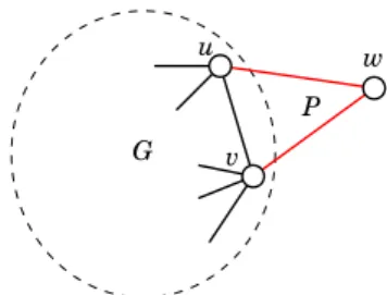
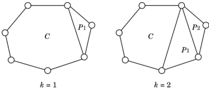
(2) Vol.2014-AL-147 No.14 2014/3/4. IPSJ SIG Technical Report. 1 ([4], [5]) For k ∈ {1, 2}, n ≥ 2k + 1, γk (G) ≤ ⌊ Corollary ⌋ n for a maximal outerplanar graph G of n nodes. 2k+1 ⌊ ⌋ n Proof. It is trivial for n = 3, 4. Consider n ≥ 5. Let p = 2k+1 and r = n − p(2k + 1). Notice that 0 ≤ r ≤ 2k ≤ 4. It is easy to see that any maximal outerplanar graph with four or more nodes must have a simple ear on the outer boundary, removing which we get a maximal outerplanar graph with one fewer nodes. Repeating this argument, we see G = G0 + P1 + · · · + Pr for some maximal outerplanar graph G0 of p(2k+1) = n−r nodes, and simple ears Pi on the outer boundary of Gi−1 = G0 +· · ·+Pi−1 , i = 1, . . . , r (the decomposition may not by unique). Since G0 is a maximal outerplanar graph, its outer boundary is a Hamilton cycle. Clearly P1 is a simple ear with respect to C too, and the outer boundary of graph G′1 = C + P1 is the same as the outer boundary of G1 . Repeating the argument, we see Pi is a simple ear with respect to graph G′i−1 = C + · · · + Pi−1 too, and the outer boundary of G′i = G′i−1 + Pi is the same as the outer boundary of Gi , i ≥ 2. See an illustration in Fig. 3.. P1 C. P2 C P1. k=1. k=2. Fig. 3 An illustration for Corollary 1: k = 1, 2 cases for graph G3 in Fig. 1, where the inner⌊ edges that ⌋ belongs to G0 − C are not shown. ⌋ ⌊ Notice n n C has (2k + 1) 2k+1 nodes and there are n − (2k + 1) 2k+1 ears.. Now by Theorem 1, we have γk (G′r ) ≤ p. Since graph G = Gr has the same node set as G′r but with ⌊ a ⌋superset of edges, it is n obvious that γk (G) ≤ γk (G′r ) ≤ p = 2k+1 . □ Corollary 2 ([4] for the k = 1 case) For a maximal outerpla⌊ ⌋ n nar graph with n nodes, a k-domination set of size at most 2k+1 can be found in O(n) time if k = 1, 2. Proof. In the above proof for Corollary 1, a decomposition G = G0 + P1 + · · · + Pr can be found in O(n) time simply by repeatedly finding degree two nodes and maintaining the degrees with a bucket. On the other hand, determining the Hamilton cycle C for G0 requires O(n) time (see [3]). Finding a k-domination set for G′r , which is also a k-domination set for G, requires O(n) time by Theorem 1. Therefore the total running time is O(n). □ Remark We remark that Theorem 1 is stronger than the results in [4], [5]. Graph G1 in Fig. 1 is a simple example.. Therefore in a graph G, a set D of nodes is a k-domination set if and only if distG (D, v) ≤ k for all nodes v. 2.1 Case r = 0 (a cycle C of p(2k + 1) nodes with no ear) Let C be a simple cycle of p(2k + 1) nodes v1 , v2 , . . . , v p(2k+1) . Obviously γk (C) = p. In fact, there are exactly 2k + 1 size-p k-domination sets for C: { } S i = vi , v2k+1+i , . . . , v(p−1)(2k+1)+i , i = 1, 2, . . . , 2k + 1. Output any one of S i requires O(n) time. 2.2 A glance at the proof for r ≥ 1 First notice that the distance labels for two neighbor nodes u and u′ on C can have only three relations: ( 1 ) distC (S i , u) = distC (S i , u′ ) = k, ( 2 ) distC (S i , u) − distC (S i , u′ ) = −1, ( 3 ) distC (S i , u) − distC (S i , u′ ) = 1, and we can (uniquely) determine S i in all of these relations. We observe that adding a simple ear P to cycle C may result some S i infeasible to C + P but there can be only one of them. We conjecture that, for all r ≤ 2k, adding r ears ⌊ can ⌋ result at most n r of these sets S i infeasible, thus γk (G) ≤ 2k+1 holds for all k (because there are 2k + 1 > r sets of S i ). The idea is to determine the number of sets S i that k-dominate C + P1 + · · · + Pr−1 but not C + P1 + · · · + Pr . So far, we could only prove for r ≤ 4, thus γ1 (G) and γ2 (G) only, as shown in the following subsections. 2.3 Case r = 1 (one ear) Suppose that an ear P1 = u1 − w1 − u′1 is added to C and node w1 is not k-dominated by some S i . Clearly this can happen only if distC+P1 (S i , u1 ) = distC+P1 (S i , u′1 ) = k, thus distC (S i , u1 ) = distC (S i , u′1 ) = k, hence S i can be uniquely determined. There are still (2k + 1) − 1 = 2k ≥ 2 sets S j ( j , i) that can k-dominate C + P1 . Thus the case r = 1 is shown. 2.4 Case r = 2 (two ears) We have shown that there are 2k sets S j that can k-dominate C + P1 . Let S i be the one that cannot k-dominate C + P1 . Now suppose an ear P2 = u2 − w2 − u′2 is added to C + P1 . Clearly if P2 is an ear with respect to C too (i.e., w1 < {u2 , u′2 }) then we are done, since, by the argument for r = 1, P2 can result at most one more S j , j , i, infeasible to C + P1 + P2 . Thus we only need to consider when w1 ∈ {u2 , u′2 }. Without loss of generality, assume u2 = w1 and u′2 = u′1 . See Fig. 4. u1. u’2. w2 P2. u1. P1 u2. C. C. 2. Proof for Theorem 1 Let distG (u, v) denote the distance between nodes u and v in a graph G, which is the minimum number of edges required to connect u and v in G. Given a node set D, let distG (D, v) denote the distance between D and a node v, i.e., distG (D, v) = min {dist(u, v)} . u∈D. c 2014 Information Processing Society of Japan ⃝. w1=u2. w1. P2 w2. u’1 Fig. 4. u’1=u’2. Illustrations for Case r = 2: In the left sub-case, P1 and P2 are ears with respect to C; In the right sub-case, only P1 is an ear with respect to C (P2 is an ear with respect to C + P1 in both sub-cases).. Assume that w2 is not k-dominated by some set S h (h , i) that 2.

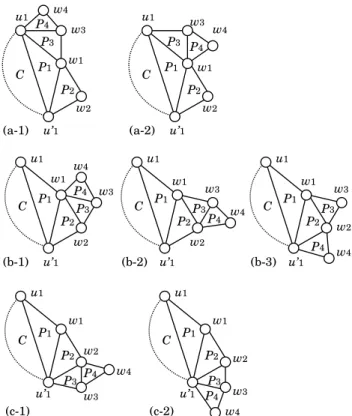
(3) Vol.2014-AL-147 No.14 2014/3/4. IPSJ SIG Technical Report. k-dominates C +P1 . This can happen only if distC+P1 +P2 (S h , u2 ) = distC+P1 +P2 (S h , u′2 ) = k. Hence we have distC+P1 +P2 (S h , u′1 ) = k and distC+P1 +P2 (S h , u1 ) = k − 1. Therefore S h can be uniquely determined. Thus we have at least 2k − 1 ≥ 1 sets S j ( j < {i, h}) that k-dominates both w1 and w2 , hence C + P1 + P2 . Determining the sub-case and, if necessary, S h , requires O(1) time, hence the running time for case r = 2 is O(n) too. For k = 1, since 0 ≤ r ≤ 2k = 2, the proof finishes here. For k ≥ 2, we need to consider the cases r = 3, 4 further.. u1. C. w4 P4 w3 P3 w1 P1. u1. w3. P1. C. P2 w2. u’1. w2 u’1. (a-2). u1. u1. u1. w4 w1. 2.5 Case r = 3 (three ears) So far we showed that adding two ears P1 and P2 can result at most two of the 2k + 1 sets S 1 , S 2 , . . ., S 2k+1 infeasible to C +P1 +P2 . Now we show that adding a third ear P3 = u3 −w3 −u′3 to C + P1 + P2 can result at most one more S i infeasible to C + P1 + P2 + P3 . This will prove case r = 3 since (2k + 1) − 3 > 0. Consider the two sub-cases for r = 2 (see the illustration in Fig. 4). In the first sub-case, P1 and P2 are both ears with respect to C. Then obviously repeating the argument for case r = 2 shows the claimed result. Thus we only need to consider the sub-case that P2 is not an ear with respect to C. Then, again we are done if P3 is an ear with respect to C. Therefore finally the non-trivial sub-cases happen only when P3 is on the u1 − w1 − w2 − u′1 path, which are shown as sub-cases (a), (b) and (c) in Fig. 5. u1. u1. u1. w3 P3 C. P1. w1. w1 C. P1 P3. P2. u’1 Fig. 5. C. P1. P2 w2. (a). w1. w3. P2. w2 (b). u’1. w2. P3 (c). u’1. w3. Illustrations for the non-trivial sub-cases for r = 3.. Again assume that w3 is not k-dominated by some S ℓ among the 2k − 1 (or more) S j that k-dominate C + P1 + P2 . In sub-case (a), this can happen only if distC+P1 +P2 +P3 (S ℓ , u1 ) = distC+P1 +P2 +P3 (S ℓ , w1 ) = k, hence distC+P1 +P2 +P3 (S ℓ , u′1 ) = k − 1. Therefore set S ℓ can be uniquely determined. Sub-case (b) is almost the same (notice u1 and u′1 cannot have distance labels k − 1 at the same time). In sub-case (c), distC+P1 +P2 +P3 (S ℓ , u′1 ) = distC+P1 +P2 +P3 (S ℓ , w2 ) = k implies distC+P1 +P2 +P3 (S ℓ , w1 ) = k − 1, hence distC+P1 +P2 +P3 (S ℓ , u1 ) = k − 2, impossible. The running time is obviously O(n). 2.6 Case r = 4 (four ears) We showed that there can be at most three of S i infeasible to C + P1 + P2 + P3 . Now we prove that adding a forth ear P4 = u4 − w4 − u′4 can result at most one more infeasible. In fact, the non-trivial (i.e., requires diﬀerent argument other than what we have used for r ≤ 3) sub-cases happen only when P4 is on the outer boundary of C + P1 + P2 + P3 consisting of nodes u1 , w1 , w2 , w3 and u′1 (see Fig. 5), as shown in Fig. 6. Assume that w4 is not k-dominated by some S q among the 2k − 2 (or more) S j that k-dominate C + P1 + P2 + P3 . This can happen only if distC+P1 +···+P4 (S q , u4 ) = distC+P1 +···+P4 (S q , u′4 ) = k. Then c 2014 Information Processing Society of Japan ⃝. w1. P2. (a-1). C. w1 P4 w3 P3. P1. C. P3 P2. w2 u’1. (b-2). P2. w2. P4 w4. u’1. (b-3). w1. u’1. w1 C. P2 w2 P4 P3 w3. (c-1) Fig. 6. w4. w3 P3. u1. P1. u’1. P4. C. P1. w2. u1. C. w1. w3. P1. P2. (b-1). w4. P3 P4. P1 P2. w2. w4 P3 u’1 P4 w3 w4 (c-2). Non-trivial non-symmetric sub-cases for r = 4. (a-*), (b-*), (c-*) are derived from sub-cases (a), (b), (c) in Fig. 5, respectively, by adding P4 to the outer boundary consisting of u1 , w1 , w2 , w3 and u′1 .. we can calculate distC+P1 +···+P4 (S q , u1 ) and distC+P1 +···+P4 (S q , u′1 ). Easy calculation shows that only sub-case (b-2) has a unique feasible distance labeling distC+P1 +···+P4 (S q , u1 ) = k − 2 and distC+P1 +···+P4 (S q , u′1 ) = k − 1. Such a set S q does not exist in other sub-cases. Clearly the total running time is O(n), proving Theorem 1. □. 3. Conclusion and future work. ⌊ ⌋ n In this paper, we gave a simple proof to show γk (G) ≤ 2k+1 , k = 1, 2, for a maximal outerplanar graph G of n nodes with a linear-time algorithm. We conjecture that the bound holds for all k. Currently we are working on a simpler proof for r ≥ 5 with fewer case-studies (or to develop a counter example). Finally we remark that our technique can be used to improve the results for guarding numbers and vertex cover numbers in [5]. Acknowledgments This work was supported by JSPS KAKENHI Grant Numbers 23700018, 25330026, and John-man Program of Kyoto University. References [1] [2] [3] [4] [5]. Diestel, R.: Graph Theory, Springer-Verlag, pp. 107 (2000). EIGindy, Hossam A.: Hierarchical decomposition of polygons with applications, PhD. thesis, School of Computer Science, University of McGill (1985). Mitchell S., Beyer T., and Jones W.: Linear Algorithms for Isomorphism of Maximal Outerplanar Graphs, Journal of the ACM, Vol. 26, Issue 4, pp. 603–610 (1979). Matheson L.R., and Tarjan R.E.: Dominating Sets in Planar Graphs, European Journal of Combinatorics, Vol. 17, Issue 6, pp. 565–568 (1996). Canales S., Hernandez G., Martins M., and Matos I.: Distance domination, guarding and vertex cover for maximal outerplanar graph, arXiv:1307.2043 [cs.CG] (2013).. 3.

(4)