A module system
with applicative functors
and recursive path references
Abstract
When developing a large software program, it is useful to decom-pose the program into smaller parts and to reuse them in different contexts. Many modern programming languages provide some forms of module systems to facilitate such factoring of programs.
The ML module system is well-known for its flexibility in program structuring. A programmer can factor programs into hierarchy using nested structures and can define functors, which are functions over modules, to reuse program codes. Moreover, signatures, which repre-sent types of modules, allow the programmer to control abstraction of modules. In spite of this flexibility, modules cannot be defined recur-sively in ML, since dependencies between modules must accord with the order of definitions. A complex program may be naturally decom-posed into recursive modules. Yet, this constraint of ML will force the programmer to consolidate conceptually separate components into a single module, intruding on modular programming.
Introducing recursive modules is a natural way out of this predica-ment. Existing proposals, however, vary in expressiveness and ver-bosity. In this paper, we propose a type system for recursive modules, which can infer their signatures. Opaque signatures can also be given explicitly, to provide type abstraction either inside or outside the re-cursion. The type system is decidable, and is sound for a call-by-value semantics.
Acknowledgment
Jacques Garrigue strongly supported me throughout my work. We have had dense and fruitful discussions regularly and he gave me many many many useful suggestions and never discouraged my premature ideas. He always listened to me carefully and gave me appropriate advice and references. Our discussions were not limited to about recursive modules but about various topics on programming languages. All these discussions were exciting and useful to my work. I cannot thank him enough for his support.
Masahito Hasegawa supported me throughout my work. He supported me both technically and spiritually during my study at RIMS. Although our work is not closely related, he understood my work and gave me useful suggestions. In particular, his advice from a more technically fundamental point of view often made my thought clearer. I thank him very much.
Susumu Nishimura gave me useful suggestions on my work. He also care-fully read my draft papers and gave me comments, which greatly helped me improve the drafts. I thank him very much.
Declaration
I declare that this work is entirely written by myself. The result presented in Part I is motivated by my previous work [48] and extends it from a technical point of view. The result of this whole thesis is condensed in [47], where proof and details are omitted.
Contents
I
Introduction
9
II
Abbreviation expansion for recursive modules
18
1 Example 20
2 Syntax 25
3 Module path expansion 29
3.1 Module path expansion algorithm . . . 33
3.1.1 Ground expansion . . . 33
3.1.2 Well-definedness and termination . . . 36
3.2 Variable normalization . . . 37
3.3 Termination and well-definedness of the module path expansion . . . 38
4 Type expansion 40 4.1 Type expansion algorithm . . . 40
4.2 Well-definedness and termination . . . 45
5 Typing 47 5.1 Type equality . . . 47
5.2 Core type reconstruction . . . 47
5.3 Typing rules . . . 50
6 Soundness 55 6.1 Proof of the soundness . . . 56
7 Type inference for the core language 66
III
Recursive modules for programming
67
9 Syntax 73
9.1 Elaboration . . . 75
10 Reconstruction 81 10.1 Lazy module types . . . 81
10.2 Look-up . . . 83
10.3 Expansion algorithms . . . 87
10.4 Lazy program type reconstruction . . . 93
11 Type-correctness check 98 11.1 Type equality . . . 98
11.2 Typing rules . . . 99
12 Soundness 105 12.1 Proof of the soundness . . . 107
12.1.1 Results from Marguerite . . . . 107
12.1.2 Type system TraviataX . . . . 109
12.1.3 From Traviata to TraviataX . . . . 125
13 The expression problem 132
IV
Discussions
137
14 Related work 137 14.1 Type systems . . . 137 14.2 Initialization . . . 140 14.3 Mixin modules . . . 140 15 Future work 142 15.1 Separate type checking and compilation . . . 14215.2 Lazy modules . . . 142
15.3 Relaxing the first-order structure restriction . . . 143
15.4 The double vision problem . . . 143
List of Figures
1 A Set module for integer sets . . . 10
2 A FSet functor for a parameterized set module . . . 10
3 A AFSet functor, whose body is ascribed by a signature . . . 11
4 An extension of the AFSet functor . . . 14
5 Tree and forest . . . 21
6 A signature for Tree and Forest . . . 22
7 Syntax for the module language . . . 26
8 Syntax for the core language . . . 27
9 Notation convention . . . 31
10 Look-up . . . 31
11 A program P1 . . . 31
12 Module path expansion . . . 33
13 Ground expansion . . . 35
14 Variable normalization . . . 38
15 Type expansion . . . 41
16 Type equivalence . . . 48
17 Type equivalence on located types . . . 48
18 Type reconstruction . . . 49
19 Datatype look-up . . . 49
20 Typing rules . . . 51
21 Typing for the core language . . . 52
22 Well-formed module paths . . . 52
23 Realization . . . 53
24 Normalization of module paths . . . 56
25 Unsafe ground-normalization . . . 57
26 Tree and Forest with structural recursive types . . . 68
27 Taking the fix-point of a functor . . . 69
28 Modules for trees and forests . . . 72
29 The module language of Traviata . . . . 74
30 Syntax for module paths . . . 74
31 The core language of Traviata . . . . 74
32 The module language after elaboration . . . 76
33 Module paths after elaboration . . . 76
34 Example of elaboration . . . 78
35 Result of elaboration . . . 78
37 Lazy module types . . . 82
38 Notation convention . . . 83
39 Look-up . . . 84
40 Self variable environments of module descriptions . . . 84
41 A program P1 . . . 86
42 Look-up for type and value paths . . . 87
43 Location equivalence . . . 88
44 Ground expansion . . . 90
45 Variable normalization . . . 91
46 Module path expansion . . . 91
47 Type expansion . . . 92
48 Core type reconstruction . . . 94
49 Datatype look-up . . . 94
50 Lazy program type reconstruction . . . 95
51 Manifestation of type specifications . . . 96
52 Type equivalence . . . 99
53 Equivalence on located types . . . 99
54 Equivalence on module paths in located forms . . . 99
55 Typing rules for the module language . . . 100
56 Typing rules for the core language . . . 101
57 Subtyping . . . 102
58 Well-formed module paths . . . 102
59 Realization . . . 103
60 Erasure look-up . . . 106
61 Sealing erasure . . . 106
62 Small step normalization of module paths . . . 107
63 Normalization of module paths in Traviata . . . . 109
64 A small step reduction of types . . . 110
65 Typing rules for the module language in TraviataX . . . 112
66 Typing rules for the core language in TraviataX . . . . 113
67 Located form judgment . . . 113
68 Datatype look-up in TraviataX . . . 114
69 Subtyping in TraviataX . . . . 114
70 Well-formed module paths in TraviataX . . . . 115
71 Realization in TraviataX . . . . 115
72 Erasure look-up for value paths . . . 122
73 Full manifestation of type specifications . . . 126
75 Instantiation of module expressions . . . 129
76 A first language . . . 133
77 A second language . . . 134
78 To merge independantly developed extensions . . . 136
79 Example of O’Caml applicative functors . . . 138
80 Weakness of applicative functors in O’Caml . . . 138
Part I
Introduction
The ML module system
When developing a large software program, it is useful to decompose the pro-gram into smaller parts and to reuse them in different contexts. Module sys-tems play an important role in facilitating such factoring of programs [29, 5]. Many modern programming languages provide some forms of module sys-tems. Examples are class systems in object-oriented languages, the package mechanism in Java and the ML module system.
The family of ML programming languages, which includes Standard ML [46, 45] (hereafter, SML) and Objective Caml [42] (hereafter, O’Caml), provides a powerful mechanism for modular development of large programs, namely the ML module system [44, 40, 52]. Three important features of the module system are nested structures, functors and signature ascription. Here we in-troduce them by gradually extending a small example program in an attempt to build a versatile set module.
Nested structures Modules can be nested. That is, they can contain definitions of modules, in addition to definitions of types and core ex-pressions. Hence they allow hierarchical decomposition of programs. In Figure 1, we define a Set module representing sets of integers. We pack into the Element sub-module type and value components that are relevant to elements of those integer sets. Observe that module hierarchy also allows namespace management. The Element module contains a type component named t, which represents the type of ele-ments held in sets; the Set module contains a type component of the same name, which represents the type of sets. A programmer can dis-tinguish between these two components of the same name by referring to the former as Set.Element.t and the latter as Set.t. The ML scop-ing rule for backward references allows us to use Element.t to refer to Set.Element.t in the definition of Set.t 1
1Precisely, we cannot use Set.Element.t in the definition of Set.t or Set.sum. This amounts to forward references, that the current ML module system does not allow.
module Set = struct
module Element = struct type t = int
val unit = 0
val add x y = x + y end
type t = Element.t list val empty = []
val sum l = case l with [] ⇒ Element.unit
| hd :: tl ⇒ Element.add hd (sum tl) end
Figure 1: A Set module for integer sets
module FSet =
functor(X : sig type t val unit : t val add : t → t → t end) → struct
module Element = X type t = Element.t list val empty = []
val sum l = case l with [] ⇒ Element.unit
| hd :: tl ⇒ Element.add hd (sum tl) end
module AFSet =
functor(X : sig type t val unit : t val add : t → t → t end) → (struct
module Element = X type t = Element.t list val empty = []
val sum l = case l with [] ⇒ Element.unit
| hd :: tl ⇒ Element.add hd (sum tl)
end : sig type t val empty : t val sum : t → X.t) module ASet = AFSet(Set.Element)
Figure 3: A AFSet functor, whose body is ascribed by a signature
Functors Functors are functions over modules, where their formal param-eters are explicitly annotated with signatures. Signatures are types of modules. The body of a functor can refer to a component of the parameter as long as the parameter’s signature says that it has this component. Functor application instantiates modules, where argument modules must implement all the components that the signature of the parameter requires and determine the behavior of the resulting mod-ules. Functors are useful to ease code reuse.
In Figure 2, we define a functor FSet, a functorized version of the above Set module. When applied, FSet instantiates a module representing sets whose element type is determined by the argument module. In-deed, we can instantiate an equivalent of the above Set module by applying FSet to Set.Element, i.e., FSet(Set.Element).
Signature ascription Modules can be ascribed by signatures. A signature does not have to mention all the components that the ascribed module contains but may only specify some of them translucently [27, 37, 43]. Thus a programmer can flexibly control accessibility of module compo-nents. Signatures improve modularity of programs.
In Figure 3, we define a functor AFSet by ascribing the above FSet functor with a signature. The signature abstracts away the underlying representation of sets and hides the sub-module Element. We can in-stantiate a module for integer sets by applying AFSet to Set.Element,
as we do for defining the module ASet. Due to the signature ascription, ASet.empty is the only value of type ASet.t that we can build. In spite of this flexibility, the ML module system does not allow recursive modules. In ML, module dependencies must accord with the definition order. For instance, we cannot define the function sum before the Element sub-module in Figure 1. Thus a programmer cannot define recursive functions or types across module boundaries. The absence of recursive modules is a major disadvantage of the ML module system, when compared to object-oriented languages, like Scala [1] and Java. These languages have supported recursive definitions across class boundaries from the beginning, and this feature is heavily used in practice.
The ML programming language enjoys strong type safety. Yet, due to the lack of recursive modules, a programmer may have to consolidate con-ceptually separate components into a single module, intruding on modular programming [56]. If ML had both recursive modules and this flexible mod-ule language, the programmer could enjoy a strongly type safe programming language with an equally strong expressive power.
Recently, much work has been devoted to investigating extensions with recursion of the ML module system. There are at least two important issues involved in recursive modules, namely initialization and type checking.
Initialization: Suppose that a programmer can freely refer to value
com-ponents of structures forward and backward. Then he might carelessly de-fine value components cyclically like val l = m val m = l. Initialization of modules having such cyclic value definitions would either raise a runtime error or cause meaningless infinite computation. Boudol [6], Hirschowitz and Leroy [34, 33, 31, 32], and Dreyer [15] examined type systems which ensure safe initialization of recursive modules. Their type systems ensure that the initialization does not attempt to access undefined recursive variables. The above cyclic definitions will be rejected by their type systems because ini-tialization of the value component l requires an access to itself. This path is not the main focus of this thesis.
Type checking: Designing a type system for recursive modules is another
important and non-trivial issue; this is the main focus of this thesis. Sup-pose that a programmer can layout modules in any order regardless of their dependencies. Then, it might happen that a function returns a value whose type is not yet defined at the point where the function is defined. To type
check the function, a type system should somehow know about the type, which is going to be defined in the following part of the program.
Type checking recursive modules
To type check recursive modules, existing proposals [11, 56, 16, 41] rely on signature annotations from a programmer. The programmer has to assist the type checker by writing enough type information so that recursive modules do not burden the type checker with forward references.
The amount of required annotations varies in each proposal and depends on where to enforce type abstraction. In the context of recursive modules, a programmer can enforce type abstraction inside the recursion by giving sig-natures individually to modules, or outside the recursion by writing a single signature for the whole recursive modules. In all proposals, a programmer has to write two different signatures for the same module to enforce abstrac-tion outside the recursion; one of the signatures is solely for assisting the type checker and does not affect the resulting signature of the module. Moreover, due to the annotation requirement a programmer cannot use type inference during development. This is unfortunate since a lot of useful inference algo-rithms have been and will be developed to support smooth development of programs.
Even if we write annotations for recursive modules, this still leaves two subtle issues to be considered.
Cyclic type specifications in signatures
To annotate recursive modules with signatures, existing type systems allow some forms of recursive references between signatures. To develop a practical algorithm for judging type equality, one may want to ensure that manifest type specifications in signatures do not declare cyclic types. For instance, one may want to forbid programmers from writing the following cyclic signature:
sig type t = s type s = t end
Detection of cyclic type specifications is not a trivial task when the mod-ule language supports both applicative functors [38, 18] and recursive sig-natures, as O’Caml does. Applicative functors give us more flexibility in expressing type sharing constraints between modules by allowing type paths to contain functor application. For instance, with functors being applicative
module EAFSet =
functor(X : sig type t val unit : t val add : t → t → t end) → (struct
module Set = AFSet(X) include Set
val total l = case l with [] ⇒ Element.unit
| hd :: tl ⇒ Element.add (Set.sum hd) (total tl) end : sig
type t = AFSet(X).t val empty : t val sum : t → X.t val total : t list → X.t
end)
Figure 4: An extension of the AFSet functor
AFSet(Set.Element).t is a valid type in Figure 3. We can further extend the AFSet functor with a new function total, preserving type equality with AFset as shown in Figure 4. While applicative functors are useful, there is the potential that a programmer may carelessly write cyclic type specifica-tions by combining applicative functors and recursive signatures, in such way that a na¨ıve check cannot detect the cycle. Here is one pathological example.
module F
: functor(X : sig type t end) → sig type t = F(F(X)).t end = functor(X : sig type t end) → sig type t = F(F(X)).t end Compare the above functor definition with the definition below.
module G
: functor(X : sig type t end) → sig type t = G(X).t end = functor(X : sig type t end) → sig type t = G(X).t end On the one hand, a type system would easily detect the latter cycle, since the unrolling of the type G(X).t would be exactly G(X).t. On the other hand, the former cycle is more difficult to detect, since the unrolling of the type F(F(X)).t would yield the following infinite rewriting sequence.
F(F(X)).t → F(F(F(X))).t → F(F(F(F(X)))).t → ...
Observe that this sequence is not merely cyclic, but produces types of ar-bitrary long length. In fact, O’Caml type checker diverges for the former functor definition of F, since it attempts to build this infinite sequence inter-nally in an attempt to detect cycles.
The situation could become harder, if one wants to keep recursive defini-tions like:
module H
: functor(X : sig type t type s end) →
sig type t = H’(H’(X)).t type s = X.s → X.s end = functor(X : sig type t type s end) →
struct type t = H’(H’(X)).t type s = X.s → X.s end and H’
: functor(X : sig type t type s end) →
sig type t = X.t ∗ X.t type s = H(H(X)).s end = functor(X : sig type t type s end) →
sig type t = X.t ∗ X.t type s = H(H(X)).s end
Neither H nor H’ contains cycles. Hence, from the programmer’s perspective, there would be no reason to disallow them.
The three examples we have seen are simple. Hence one may easily distin-guish between them, judging that only the last one is legal. When recursive modules define more complex types, however, this issue becomes harder to decide.
Potential existence of cyclic type definitions
Another subtle issue involved in recursive modules is how to account for the potential existence of cyclic type definitions in structures, when their imple-mentations are hidden by signatures. For instance, should a type checker reject the program below?
module M = (struct type t = N.t end : sig type t end) and N = (struct type t = M.t end : sig type t end)
On the one hand, one could argue that this is unacceptable since the under-lying implementations of the types M.t and N.t make a cycle. On the other hand, one could argue that this is acceptable since, according to their signa-tures, the types M.t and N.t are nothing more than abstract types. Hence the modules M and N need not be accused of defining cyclic types. At least, one could argue that potential cycles in type definitions are acceptable, if the type system is still sound and decidable and this choice has merits over the other choice.
Existing type systems take different stands on this issue.
recursive modules, in which implementations of types other than datatypes cannot be hidden. Thus cyclic type definitions are never hidden by signa-tures. At the same time, a programmer cannot enforce type abstraction inside recursive modules.
Dreyer’s work [16] focuses on type abstraction inside recursive modules. He requires the absence of cyclic type definitions whether or not they are hidden inside signatures. To ensure the absence of cycles without peeking inside signatures, he puts a restriction on types whose implementation can be hidden. As a consequence, the use of structural types is restricted. For instance, his type system would reject the following program, which uses a polymorphic variant type [24] and a list type to represent trees and forests, re-spectively. (Here we use a polymorphic variant type, which is supported only in O’Caml, since the core language we want to support is that of O’Caml. Yet, a similar restriction could arise in the context of SML, when one at-tempts to use a record type to represent trees.)
module Tree = (struct
type t = [ ‘Leaf of int | ‘Node of int * Forest.t ] end : sig type t end)
and Forest = (struct
type t = Tree.t list end : sig type t end)
By replacing the polymorphic variant type with an usual datatype, one can make this program typable in Dreyer’s system. Polymorphic variant types, however, have their own merits that datatypes do not have.
The path O’Caml chose is a more liberal one. It does not care about potential cycles in type definitions, as long as signatures do not specify cy-cles. The type checker will report an error when signatures contain cyclic type specifications. (The type checker can diverge since, as we mentioned above, recursive modules and applicative functors together make it difficult to detect cycles in a terminating way.) O’Caml has a very expressive core language, whose constructs include structural types such as object types [54] and polymorphic variant types. Moreover, the path it chose keeps flexibility in using these types and in abstracting them away by signatures.
Our proposal of a type system for recursive modules
The goal of our work is to make recursive modules an ordinary construct of the module language for ML programmers. We want to use them easily in
everyday programming, possibly combining with other constructs of the core and the module languages. With this goal in mind, we propose in this thesis a type system for recursive modules which overcomes as much of the diffi-culties discussed above as possible. Concretely, we follow the path O’Caml chose but extend it by 1) enabling type inference; 2) providing a terminating procedure to detect cyclic type specifications, in the presence of applicative functors; 3) formalizing the type system and proving its soundness, but al-lowing the potential of cyclic type definitions hidden inside signatures, thus leaving flexibility in using structural types. At the current stage, we con-fine ourselves to first-order functors. We defer it to future developments to accommodate higher-order functors.
The rest of this thesis is organized into two parts in the following way. Part II We tackle the first two of the aforementioned difficulties in typing
recursive modules, that is, type inference and detection of cycles in type specifications. For a formal study, we design a calculus, named
Marguerite, which supports recursive modules and applicative functors
but does not signature ascription. We develop “expansion algorithms” which can resolve recursive references between modules by tracing mod-ule and type abbreviations. These algorithms are terminating; they will either output the result of the expansion or raise an error when they cannot prove that input recursive modules do not contain cyclic or dangling type specifications. Using these algorithms, we design a type system for Marguerite and prove that the type system is decidable and sound for a call-by-value operational semantics.
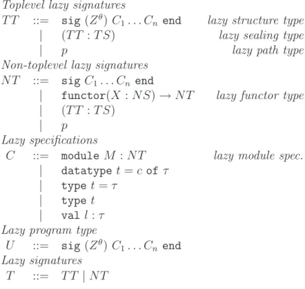
Part III We extend Marguerite with signature ascription to make the module language full-fledged. The extended language is named
Travi-ata. We reformulate the type system of Marguerite for TraviTravi-ata. The
resulting type system is two-phased, that is, it consists of a type recon-struction part and a type-correctness check part. The former part is an application of the result of Part I; the latter corresponds to a standard type checking of modules. We prove the type system is still decidable and sound.
Part II
Abbreviation expansion for
recursive modules
In this part, we focus on developing “expansion algorithms” for resolving re-cursive references between modules. The motivation of the algorithms are to reduce types into canonical forms for judging type equality. One can think of canonical forms of types as abbreviation-free types that are obtained by re-placing abbreviations with their definitions. To expand types, the algorithms trace abbreviations. Yet we have to be careful to keep them terminating, since the source program may contain dangling or cyclic abbreviations. The algorithms may raise an error when they cannot prove that both the input type and the source program do not contain dangling or cyclic references.
Every type has a unique canonical form, in which all references are re-solved. The type system judges type equality by reducing types into canon-ical forms using the expansion algorithms and by comparing their syntactic equality. For decidability of type checking, termination of the algorithms is critical.
We design the expansion algorithms to be terminating independently of well-typedness of the source program. We cannot rely on well-typedness to keep the algorithms terminating, since we need a type equality judgment to type check the program and our type equality judgment requires types to be in canonical form. The algorithms are developed separately from the type system and proved to be terminating for any input.
This separation has the following two useful consequences.
1. Typing rules are kept straightforward. This is particularly useful to extend the type system later with more expressive language constructs. These new constructs may be accompanied by rather complex typing rules, so we would like to add them without polluting their typing rules with specifics to the expansion algorithms.
2. It is easy to accommodate a possible extension of the algorithms, that is, when we come up with cleverer expansion algorithms we can replace the current ones with the new ones without or with little change in typing rules.
For a formal study, we design in this part a calculus, named Marguerite, which supports nested recursive structures and applicative functors.
Mar-guerite does not support signature ascription, on which we focus in the next
part of this thesis. In this part, we explain the expansion algorithms in de-tail and prove their termination. We present a type system for Marguerite, where the expansion algorithms play an important role in judging type equal-ity. Decidability of the type system is obtained as an immediate consequence of termination of the algorithms. We also prove a soundness result of the type system; the result includes that the expansion algorithms are consistent with the intuition for well-typed programs.
The rest of this part is organized as follows. In the next section, we overview the main features of Marguerite using an example. In Section 2, we give the syntax for Marguerite. In Section 3 and 4, we develop expansion algorithms for reducing module paths and types, respectively. In Section 5, we present the type system and in Section 6 we prove a soundness result. In Section 7, we discuss how to apply the expansion algorithms to define a core type inference algorithm.
1
Example
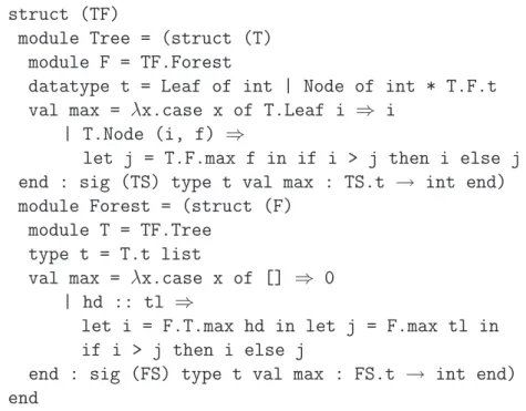
In this section, we present a scenario where recursive modules naturally arise and explain difficulties involved in type checking recursive modules, using an example given in Figure 5.
The top-level structure contains three sub-modules S, Tree and Forest, where Tree and Forest are defined in a mutually recursive way. The module S is an abbreviation for a module IntSet, which is we assume given in a library. The module Tree represents trees whose leaves and nodes are labeled with integers. The module Forest represents unordered sets of those integer trees.
To enable forward references between modules, we extend the top-level structure with an implicitly typed declaration of a self variable. Components of the top-level structure can refer to each other recursively using the self variable, regardless of definition ordering. For instance in the example, the top-level structure declares a self variable named TF, which is used inside Tree and Forest for recursive references to each other. We keep the usual ML scoping rules for implicit backward references. Thus the function Tree.split can refer to the Leaf and Node constructors without going through the self variable. It was possible to use Tree, instead of TF.Tree, inside Forest, since Tree is a backward reference for Forest. But the explicit notation seems clearer.
Let us explain the implementations of Tree and Forest in detail. Two types Tree.t and Forest.t refer to each other recursively. On the one hand, the datatype definition of Tree.t involves a type name s, which is an abbreviation for the type TF.Forest.t, a reference to the type Forest.t. On the other hand, the type Forest.t is a synonym for the type T.t list, where the type T.t is an abbreviation for TF.Tree.t, a reference to the type Tree.t. Two functions Tree.labels and Forest.labels call each other recursively. These functions calculate the sets of integers that a tree and a forest contain, respectively. Using these functions, we define the function Forest.incr, which augments a given forest only if a given tree contains original labels that are not contained in the forest.
The function split in Tree cuts off the root node of a given tree, then returns the resulting forest. The function sweep in Forest gathers leaves from a given forest. These two functions also make recursive references. The second case branch of Tree.split depends on the fact that a forest is a list of trees; Forest.sweep constructs and deconstructs trees through the
struct (TF)
module S = IntSet module Tree = struct
module F = TF.Forest type s = F.t
datatype t = Leaf of int | Node of int * s
val labels = λx.case x of Leaf i ⇒ TF.S.singleton i | Node (i, f) ⇒ TF.S.add i (F.labels f)
val split = λx.case x of Leaf i ⇒ [Leaf i] | Node (i, f) ⇒ (Leaf i) :: f
end
module Forest = struct module T = TF.Tree type t = T.t list
val labels = λx.case x of [] ⇒ TF.S.empty
| hd :: tl ⇒ TF.S.union (T.labels hd) (labels tl) val incr = λf.λt.let l1 = labels f in
let l2 = T.labels t in
if TF.S.diff l2 l1 != TF.S.empty then (t :: f) else f val sweep = λx.case x of [] ⇒ []
| (T.Leaf y) :: tl ⇒ (T.Leaf y) :: (sweep tl) | (T.Node y) :: tl ⇒ sweep tl
end end
sig (TF)
module Tree : sig type t val split : t → TF.Forest.t end module Forest : sig
type t val incr : TF.Tree.t → t → t val sweep : t → t end end
Figure 6: A signature for Tree and Forest
constructors Leaf and Node, which are declared inside Tree.
Judging type equality The main difficulty in type checking this example is in judging type equality. For instance, let us consider type checking the second branch of the function Tree.split. For the list cons operation (Leaf i) :: f to be well-typed, f must be a list of trees. In the datatype definition of Tree.t, the constructor Node is described to contain an integer and a forest. By tracing underlined four abbreviations, a type system could expand the type Tree.s into TF.Tree.t list. Then it would conclude that the list cons operation is well-typed.
In this simple well-typed example, there is clearly no potential of diver-gence in tracing abbreviations. Having both recursive modules and applica-tive functors, however, a programmer might carelessly write pathologically cyclic abbreviations which are hard to detect. Then a na¨ıve way of tracing ab-breviations may diverge, causing non-terminating type checking. In Section 3 and 4, we examine such pathological examples and develop “expansion algo-rithms” which trace abbreviations in a terminating way for reducing types into abbreviation-free forms.
Type inference To type check the example, a type system also needs to support type inference. Suppose that we want to give a signature in Figure 6 to the example, where we extend usual ML signatures with implicitly typed declarations of self variables to allow recursive references inside signatures. The signature enforces type abstraction by hiding underlying implementa-tions of the types Tree.t and Forest.t. Moreover it does not mention functions Tree.labels and Forest.labels. Since the implementation of the function Forest.incr relies on these two functions, a type system has to infer their types to type check Forest.incr.
signatures to enforce desired abstraction; one for the abstraction, which is given in Figure 6 and one for assisting the type checker, which we will examine below.
To avoid presenting too verbose signature annotations, we consider in the following examination the program in Figure 5 without the module abbrevi-ation module F = TF.Forest inside Tree. We can dispense with abbrevia-tions by replacing them with their definiabbrevia-tions; yet abbreviaabbrevia-tions are useful in practical programs [57].
To type check the example in Dreyer’s system [16] or O’Caml [42], a programmer has to write fully manifest signatures of Tree and Forest, that is, he has to present the type checker with the following signatures:
module Tree : sig
datatype t = Leaf of int | Node of int * Forest.t val labels : t → S.t
val split : t → Forest.t end
and
module Forest : sig type t = Tree.t list val labels : t → S.t
val incr : Tree.t → t → t
val sweep : t → t end
In Russo’s system [56], the self variable TF of the top-level structure must be annotated with the recursive signature below. In his system, a recursive signature contains a typed declaration of a self variable to support forward references in the signature.
sig (Z : sig module Tree : sig type t end
module Forest : sig type t = Tree.t list end end) module Tree : sig
datatype t = Leaf of int | Node of int * Z.Forest.t end module Forest : sig
type t = Tree.t list val labels : t → S.t end end
These additional signature annotations are indispensable in existing pro-posals and must be given beforehand. Then, the type checker first type checks the example assisted by these manifest signatures. Once this succeeds, type
abstraction can be enforced using the signature given in Figure 6.
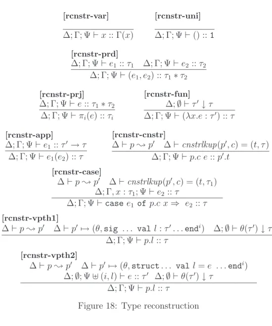
Marguerite supports type inference unlike other proposals, hence it does
not need the assistance of signature annotations. Indeed, it has an ability to reconstruct the fully manifest signatures of Tree and Forest, which the programmer has to write by himself in Dreyer’s and O’Caml type systems. This implies that the signature in Figure 6 is sufficient for Marguerite to type check the example and to enforce type abstraction together. In Section 7, we explain how we define a type inference algorithm using our abbreviation ex-pansion algorithms. In the next part of this thesis we examine and formalize how to type check the example when the signature in Figure 6 is given by the programmer.
2
Syntax
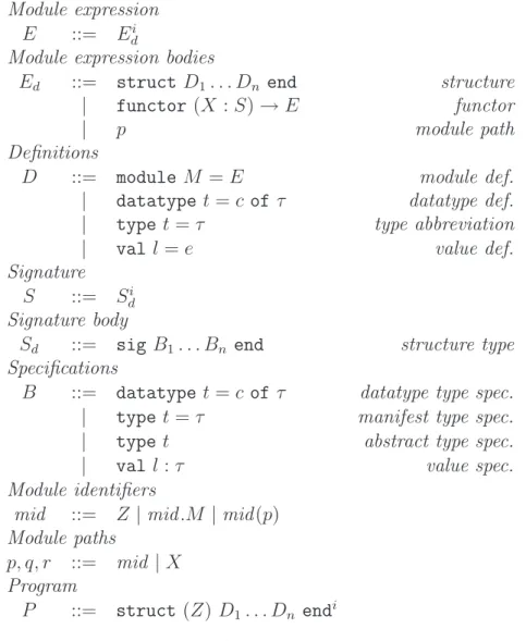
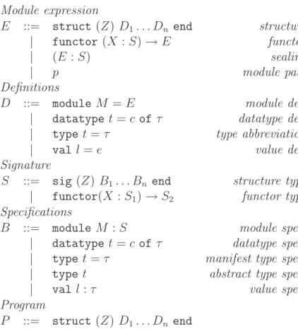
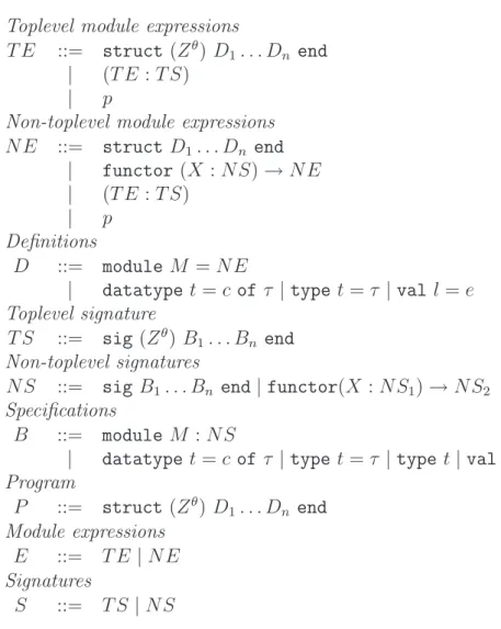
We give the syntax for the module language of Marguerite in Figure 7. It is based on Leroy’s applicative functor calculus [38]. We use M as a metavari-able for module names, X for names of module varimetavari-ables and Z for names of self variables. For simplicity, we distinguish them syntactically, however the context could tell them apart without this distinction. We also use t as a metavariable for type names, l for value names and c for constructor names. Every module expression and signature is labeled with an integer. We use these integer labels to keep expansion algorithms terminating. For instance, a module expression E is a module expression body Ed labeled with an
integer i. One can think of the integer label i of Edi as the location of Ed
in the source program. For the interest of brevity, we may omit integer labels when they are not used. For the interest of clarity, we may write additional parentheses, for instance (functor(X : sig type t end2)→ X3)1. We use metavariables i, j for integers.
A module expression body Ed is either a structure, a functor or a module
path. A structure is a sequence of module, type and value definitions. A type definition may generate a new datatype or may be an alias for another type. In particular, that structures can contain sub-modules is an important feature of the ML module system. A functor is a function over modules. Signatures for functor arguments must be given explicitly. A functor can only be applied to a module which implements the specified signature of the argument. A signature is a sequence of specifications labeled with an integer. A type specification may expose the underlying implementation of the specified type (datatype and manifest type specifications) or may hide the implementation (abstract type specification). A value is specified with its type.
A module path is a reference to a module. The flexible referencing mech-anism given by module paths is a key feature of Marguerite. A module path may refer to a module at any level of nesting within the recursive struc-ture, regardless of component ordering. Moreover, module paths can contain simple cases of functor applications, where the functor and its arguments themselves are paths. Concretely, module paths are constructed from self variables, the dot notation [9] “.M ”, which represents access to the sub-module named M of a structure, and functor applications. The syntax of module paths in Figure 7 restricts module paths not to contain paths of the forms X.M and X(p). We explain this later.
Module expression E ::= Ei
d
Module expression bodies
Ed ::= struct D1. . . Dn end structure
| functor (X : S)→ E functor
| p module path
Definitions
D ::= module M = E module def.
| datatype t = c of τ datatype def.
| type t = τ type abbreviation
| val l = e value def.
Signature S ::= Sdi Signature body
Sd ::= sig B1. . . Bn end structure type
Specifications
B ::= datatype t = c of τ datatype type spec.
| type t = τ manifest type spec.
| type t abstract type spec.
| val l : τ value spec.
Module identifiers
mid ::= Z | mid.M | mid(p) Module paths
p, q, r ::= mid | X Program
P ::= struct (Z) D1. . . Dn endi
Core types
τ ::= 1 | τ1 → τ2 | τ1∗ τ2 | p.t
Core expressions
e ::= x| () | (e1, e2)| πi(e)| (λx.e : τ) | e1(e2)
| p.c e| case e of p.c x ⇒ e | p.l
Figure 8: Syntax for the core language
For the sake of simplicity, we assume that functor applications only con-tain module paths but not structures or functors. This does not reduce the expressive power of the language [39] and we believe that in several situa-tions we can allow a larger class of functor applicasitua-tions, following Leroy’s proposal [40].
A program is a top-level structure extended with an implicitly typed dec-laration of a self variable. A self variable is bound inside the top-level struc-ture where the variable is declared. In this thesis, we only consider a bunch of recursive modules but not ordinary ones (i.e., non-recursive modules).
To develop a decidable type system, we impose a first-order structure
restriction that requires functors 1) not to take functors as arguments and
2) not to access sub-modules of arguments. The first restriction means that our functors are not higher-order, while they can still return functors. The second restriction implies that a programmer has to pass sub-modules as independent parameters to a functor instead of passing a single module which contains all the sub-modules. The restriction on the syntax of module paths is consistent with this restriction.
In Figure 8, we give the syntax for the core language of Marguerite. A core type is either a unit type 1, an arrow type τ1 → τ2, a pair type
τ1∗ τ2 or a type path p.t, which refers to a type component named t in the structure that the module path p refers to. A core expression is either a core variable (variable, for short) x, a null (), a pair (e1, e2), a projection πi(e),
an abstraction (λx.e : τ ), an application e1(e2), a value construction p.c e or deconstruction case e of p.c x ⇒ e, or a value path p.l, which refers to a value component named l in the structure that the module path p refers to.
We may say paths to mean module, type and value paths as a whole. An unusual convention is that a module variable is bound inside its own signature. For instance,
functor(X : sig type t val l : X.t end) → X is legal in Marguerite, which should be understood as
functor(X : sig type t val l : t end) → X
This convention is convenient when proving a soundness result, as the syntax of paths is kept uniform, that is, every path is prefixed by either a self variable or a module variable. In Section 13, we give an example where this convention is useful.
We write MVars(p) to denote the set of module variables contained in the module path p. We also write MVars(τ ), MVars(e) etc, with obvious meanings.
In the formalization, 1) function definitions are explicitly type annotated; 2) a path is always prefixed by either a self variable or a module variable. Our examples do not stick to these rules. Instead, we have assumed that there is an elaboration phase, prior to type checking, that adds type annotations for functions by running a type inference algorithm for the core language. The original program may still require some type annotations, to avoid running into the polymorphic recursion problem [30]. In Section 7, we discuss the details of this inference algorithm. The elaboration phase also infers omitted self variables, to complete implicit backward references.
We assume the following three conventions: 1) a program does not con-tain free module variables or free self variables; 2) all binding occurrences of module variables use distinct names; 3) any sequence of module definitions, datatype definitions, type abbreviations, value definitions, datatype specifi-cations, manifest and abstract type specifispecifi-cations, and value specifications does not contain duplicate definitions or specifications for the same name.
3
Module path expansion
In this section, we develop a module path expansion algorithm for deter-mining the module that a module path refers to. The type system uses the algorithm in the following three contexts.
1. To type check a functor application p1(p2), the type system expands p1 to make sure that p1 indeed refers to a functor definition and to dis-cover the argument signature of the functor which p2 must implement (Section 5).
2. The type expansion algorithm is defined on top of the module path expansion algorithm (Section 4).
3. The type system decides an order for type inference using the module path expansion algorithm (Section 7).
The module path expansion algorithm reduces module paths into located
forms. Intuitively, a module path p is in located form when, for all paths q
contained in p, the reference of q is already resolved. To define formally, we introduce a look-up judgment.
Look-up judgment A program environment ∆ is a mapping from a self
variable to a top-level structure and from module variables to signatures. For a program P , the program environment of P , written ∆P, is the program
environment whose domain exactly contains the self variable declared in the top-level structure of P and all module variables appearing in P and which sends the self variable to P and module variables to their own signatures specified in P . We write dom(∆) to denote the domain of ∆.
Given a module environment ∆, we define in Figure 10 a look-up judg-ment which determines the module that a given module path refers to with respect to ∆. We use θ as a metavariable for module variable bindings, which map module variables to module paths and write dom(θ) to denote the do-main of θ. The judgment ∆ ` p 7→ (θ, K) means that the module path
p resolves to the module description K, where each module variable X is
bound to θ(X) w.r.t.2 ∆. We write ² to denote the empty module variable binding, that is, a module variable binding whose domain is empty. We use
the notation convention in Figure 9. In particular, we use Kd as a
metavari-able for module description bodies, which are either module expression bodies or signature bodies, and K for module descriptions, which are either module expressions or signatures. For a module variable binding θ, θ[X 7→ p] denotes a module variable binding whose domain is dom(θ)∪ {X} and which maps
X to p and coincides with θ on dom(θ)\{X}.
Let us examine each rule of the look-up. For self variables and module variables, the judgment consults the program environment ∆. A path p.M resolves to the sub-module named M in the structure that p resolves to. Hence p1must resolve to a structure. A path p1(p2) resolves to the body of the functor that p1 resolves to, where the module variable binding is augmented with a new binding [X 7→ p2].
The look-up judgment only holds for module paths whose references are already resolved. For instance, consider the program P1 in Figure 11. Let ∆P1
be the program environment of P1, or ∆P1 = [Z7→ P1, X7→ sig type t end
3]. We have a derivation whose conclusion is:
∆P1 ` Z.M1(Z.M2).M117→ ([X 7→ Z.M2], struct end
5) but no derivation for the path Z.M3.M11.
Corresponding to the convention of the absence of free module variables in programs, we assume that any program variable environment we consider in this thesis does not contain free module variables. Precisely,
Definition 1 A program variable environment ∆ does not contain free
mod-ule variables if, for any modmod-ule path p other than modmod-ule variables, when
∆` p 7→ (θ, K) then the following two conditions hold.
1. MVars(K)⊆ dom(θ)
2. For all X in dom(θ), MVars(∆(X))⊆ dom(θ).
For a module description K, MVars(K) denotes the set of free module vari-ables in K.
Located forms Now we define located forms, which are output of the
module path expansion. A module path p is in located form if and only if p does not contain a module path which resolves to a module path according to the look-up judgment. Precisely,
Module description K ::= Kdi Module description bodies Kd ::= Ed| Sd
ss ::= struct | sig Figure 9: Notation convention
[lk-self ]
∆` Z 7→ (², ∆(Z))
[lk-mvar]
∆` X 7→ (², ∆(X))
[lk-dot]
∆` p 7→ (θ, struct . . . module M = E . . . endi)
∆` p.M 7→ (θ, E) [lk-app] ∆` p1 7→ (θ, (functor(X : S) → E)i) ∆` p1(p2)7→ (θ[X 7→ p2], E) Figure 10: Look-up struct (Z)
module M1 = (functor(X : sig type t end3)→
struct
module M11= struct end5
module M12= X6
end4)2
module M2 = struct type t = int end7
module M3 = Z.M1(Z.M2)8
end1
Definition 2 A module path p is in located form w.r.t. a program environ-ment ∆ if the following two conditions hold:
• ∆` p 7→ (θ, Ki
d) where Kd is not a module path.
• For all q in args(p), q is in located form w.r.t. ∆.
For a module path p, args(p) denotes the set of module paths appearing inside p as functor arguments. Precisely:
args(Z) =∅ args(X) = ∅
args(p.M ) = args(p) args(p1(p2)) = args(p1)∪ {p2}
We say that a module variable binding θ is in located form w.r.t. ∆ if and only if, for all X in dom(θ), θ(X) is in located form w.r.t. ∆.
The module path expansion algorithm reduces a module path into a lo-cated form or raises an error when it cannot prove that the input path does not contain dangling or cyclic references. The basic idea of the algorithm is straightforward. It traces module abbreviations until either the input mod-ule path resolves to a structure or a functor or it is reduced to a modmod-ule variable. To keep the algorithm terminating, we have to be careful about the potential existence of cyclic module abbreviations. Below we give two pathological examples which contain cycles.
To reduce notational burden, we may omit, in examples here and else-where, preceding self variables even for forward references when no ambiguity arises. Moreover, we may omit the top-level struct and end together with a declaration of a self variable.
The first example is:
module F = functor(X : sig end) → X module L = F(L)
Through the identity functor F, the definition of L makes a cycle. The second example is:
module M = M.N
This second example is more annoying than the first one, since the unrolling of M’s definition would result in the following infinite rewriting sequence, yielding module paths of arbitrary long length.
∆,∅ ` p ;g q ∆` varnlz(q) = r
∆` p ; r
Figure 12: Module path expansion
3.1
Module path expansion algorithm
We define the module path expansion in Figure 12. It is a composite of
ground expansion and variable normalization. The inference rule in Figure 12
means that the expansion reduces a given module path p into q w.r.t. a given program environment ∆, if the ground expansion reduces p into q, written ∆,∅ ` p ;g q and the variable normalization reduces q into r, written
∆ ` varnlz(q) = r. We may say that q is the located form of p when ∆` p ; q.
The ground expansion and the variable normalization are defined below. Both are terminating (Proposition 2 and 3). As a result, the module expan-sion is also terminating (Proposition 4).
3.1.1 Ground expansion
The ground expansion is ground in the sense that it does not rely on functor arguments. It either reduces a module path into a pre-located form or raises an error when 1) it cannot prove that the input module path does not contain cyclic or dangling references, or 2) the input module path does not obey the first-order structure restriction.
We first introduce pre-located forms, the central idea for defining the ground expansion. A module path p is in pre-located form if and only if p does not contain a module path which resolves to a module identifier according to the look-up judgment. Precisely,
Definition 3 A module path p is in pre-located form w.r.t. a program
envi-ronment ∆ if the following two conditions hold:
• ∆` p 7→ (θ, Ki
d) and Kd is not a module identifier. (Hence Kd can be
a module variable.)
The locution “pre-located form” indicates that we can turn a pre-located form into a located form by substituting functor arguments, as we show in Proposition 3.
We say that a module variable binding θ is in pre-located form w.r.t. ∆ if and only if, for all X in dom(θ), θ(X) is in pre-located form w.r.t. ∆.
The important feature of pre-located forms is that they satisfy a substitu-tion property, as stated in Lemma 1 below. We first define length of module paths, which we use to prove the lemma.
len(Z) = 1 len(X) = 1
len(p.M ) = 1 + len(p) len(p(q)) = len(p) + len(q)
For a module path p and a module variable binding θ, we write θ(p) to denote the module path obtained by applying the substitution θ to p. Precisely,
θ(Z) = Z θ(X) =
{
X when X 6∈ dom(θ)
p when X ∈ dom(θ) and θ(X) = p
θ(p.M ) = θ(p).M θ(p1(p2)) = θ(p1)(θ(p2))
Lemma 1 (Substitution property) Let p and θ be in pre-located form
w.r.t. ∆. Then θ(p) is in pre-located form w.r.t. ∆.
Proof. By induction on the length of p. 2
We also use the following lemma to define the ground expansion.
Lemma 2 Let p be in pre-located form w.r.t. ∆. If ∆` p 7→ (θ, K), then θ
is in pre-located form w.r.t. ∆.
Proof. By induction on the derivation of ∆` p 7→ (θ, K). 2
It is an important observation that Lemma 1 holds due to the fist-order structure restriction. If functors took nested structures as arguments, then the module path [X7→ L]X.M would not be in pre-located form in the program:
module F = functor(X : sig module M : sig end end) → struct module M = X.M end
module L = struct module N = struct end module M = N
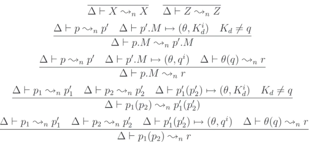
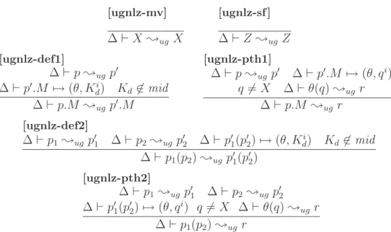
[gnlz-mvar] − ∆, Σ` X ;g X [gnlz-self ] −− ∆, Σ` Z ;g Z [gnlz-def1] ∆, Σ` p ;g p0 ∆` p0.M 7→ (θ, Ki d) Kd6∈ mid ∆, Σ` p.M ;g p0.M [gnlz-pth1] ∆, Σ` p ;g p0 ∆` p0.M 7→ (θ, qi) q 6= X ∆, Σ ] i ` q ;g r ∆, Σ` p.M ;g θ(r) [gnlz-def2] ∆, Σ` p1 ;g p01 ∆, Σ` p2 ;g p20 ∆` p01(p02)7→ (θ, Kdi) Kd6∈ mid ∆, Σ` p1(p2);g p01(p02) [gnlz-pth2] ∆, Σ` p1 ;g p01 ∆, Σ` p2 ;g p02 ∆` p01(p02)7→ (θ, qi) q6= X ∆, Σ ] i ` q ;g r ∆, Σ` p1(p2);g θ(r)
Figure 13: Ground expansion
The module variable binding [X7→ L] is in pre-located form, but the module path L.M is not (because L.M resolves to a module identifier).
We define the ground expansion in Figure 13. The judgment ∆, Σ `
p ;g q means that the ground expansion reduces the module path p into
the module path q with Σ locked w.r.t. the program environment ∆. We use Σ as a metavariable for sets of integers. The notation Σ] i means Σ ∪ {i} whenever i 6∈ Σ. We may say that q is the pre-located form of p w.r.t. ∆ when ∆, Σ` p ;g q holds for some Σ.
Observe that for any program environment ∆, module path p and lock Σ, proof search for ∆, Σ ` p ;g is deterministic, where “ ” is a place-holder.
In other words, for any ∆, p and Σ we can search a derivation tree whose conclusion is ∆, Σ` p ;g in a deterministic way. The search may fail with
no applicable rules. When it is successful, we find a module path q such that ∆, Σ` p ;g q holds. In this way, we regard the inference rules of the ground
expansion as defining an algorithm which takes ∆, p and Σ as input then either returns q when the search succeeds in building a derivation tree of ∆, Σ` p ;g q or raises an error when the search fails. We prove termination
of the proof search later in Proposition 2.
and [gnlz-self ] are straightforward. For a path of the form p.M , the ground expansion first reduces the prefix p ([gnlz-def1][gnlz-pth1]). Suppose that p0 is the pre-located form of p. Then there are two cases depending on whether
p0.M resolves to a module identifier or not. When p0.M resolves to a module
description other than a module identifier ([gnlz-def1]), then p0.M is in
pre-located form and the ground expansion terminates. When p0.M resolves to
a module identifier q ([gnlz-pth1]), then the ground expansion traces the abbreviation q. This is the key rule, hence we explain it in detail.
As a simple case, suppose that q is in pre-located form w.r.t. ∆. Then ∆, Σ] i ` q ;g q holds immediately whenever i is not in Σ (see Lemma 6)
and the ground expansion returns θ(q). By Lemma 1 and 2, we know that
θ(q) is in pre-located form. In general, q is not necessarily in pre-located
form. Hence, the ground expansion reduces q first to obtain its pre-located form in the premise ∆, Σ] i ` q ;g r, then applies the substitution θ to r.
This explains the idea of the ground expansion. It additionally holds a lock Σ during the expansion for termination. In short, when the ground expansion holds a lock Σ, then it is in the middle of reducing the module paths labeled with the integers in Σ. The rules [gnlz-pth1] and [gnlz-pth2]
have the side condition i6∈ Σ implicitly; thanks to the condition, the ground expansion avoids tracing the same module abbreviation cyclically.
The rules [gnlz-def2] and [gnlz-pth2] for paths of the form p1(p2) are similar to [gnlz-exp1] and [gnlz-pth1], respectively.
3.1.2 Well-definedness and termination
Here we prove that the ground expansion does reduce module paths into pre-located forms unless it raises an error and that it is terminating.
Proposition 1 (Well-definedness of the ground expansion) For any
pro-gram environment ∆, lock Σ and module paths p, q, if ∆, Σ` p ;g q then q
is in pre-located form w.r.t. ∆.
Proof. By induction on the derivation of ∆, Σ ` p ;g q and by case on the
last rule used. Use Lemma 1 and 2 for the rules[gnlz-pth1]and[gnlz-pth2].
2
Definition 4 A binary relation R on any set is well-founded if there is no infinitely descending sequence in R, that is, there is no sequence {ri}∞i=1such
that, for all i in 1, 2, . . ., ri R ri+1 holds.
Proposition 2 (Termination of the ground expansion) For any program
environment ∆, lock Σ and module path p, proof search for ∆, Σ ` p ;g
will terminate.
Proof. Below, we define a well-founded relation >g∆ on pairs (p, Σ) of a
module path p and a lock Σ w.r.t. ∆. It is easy to check that if ∆, Σ2 `
p2 ;g is a premise of ∆, Σ1 ` p1 ;g , then (p1, Σ1) >g∆ (p2, Σ2).
Thus, if there is an infinitely deep derivation tree of the ground expansion, then there is an infinitely descending sequence in >g∆. This contradicts
well-foundedness of >g∆. By K¨oning’s lemma on finitely branching trees, we
obtain the proposition.
(p1, Σ1) >g∆ (p2, Σ2) holds if and only if either of the following three
con-ditions holds. We write IntLabs∆ to denote the set of integer labels appearing
in ∆.
1. p1 = p01.M and p2 = p01 and Σ1 = Σ2.
2. p1 = p11(p12) and p2 = p1i with i being either 1 or 2, and Σ1 = Σ2.
3. i is not in Σ1 and Σ2 = Σ1∪ {i} ⊆ IntLabs∆
Well-foundedness of >g∆ follows from the finiteness of IntLabs∆. 2
3.2
Variable normalization
The variable normalization turns pre-located forms into located forms. In Figure 14 we define the variable normalization using two functions varnlz and varsubst. When the input module path resolves to a module variable, these functions recursively substitute for the variable the module path which is bound to the variable, according to the look-up judgment.
The proposition 3 below indicates that by combining the ground expan-sion and the variable normalization, we can calculate located forms.
Lemma 3 Let p be in located form w.r.t. ∆. If ∆ ` p 7→ (θ, K), then θ is
∆` varnlz(X) = X ∆ ` varnlz(Z) = Z ∆` varnlz(p) = p0 ∆` varsubst(p0.M ) = q
∆` varnlz(p.M) = q
∆` varnlz(p1) = p01 ∆` varnlz(p2) = p02 ∆` varsubst(p01(p02)) = q
∆` varnlz(p1(p2)) = q ∆` p 7→ (θ, Xi) ∆` varsubst(p) = θ(X) ∆` p 7→ (θ, Ki d) Kd6= X ∆` varsubst(p) = p Figure 14: Variable normalization
Proof. By induction on the derivation of ∆` p 7→ (θ, K). 2
Lemma 4 Let p be in pre-located form w.r.t. ∆. If ∆ ` p 7→ (θ, Ki
d) with
Kd 6= X and ∆ ` varnlz(p) = q, then ∆ ` q 7→ (θ1, Kdi) where, for all X in
dom(θ), ∆` varnlz(θ(X)) = θ1(X).
Proof. By induction on the length of p. Observe that by definition on the
look-up, dom(θ) = dom(θ1). 2
Proposition 3 When p is in pre-located form w.r.t. ∆, then there is a unique
q in located form w.r.t. ∆such that ∆` varnlz(p) = q.
Proof. By induction on the length of p. We show the main case.
When p = p1.M . By induction hypothesis, there is a unique p2 in located form such that ∆ ` varnlz(p1) = p2. Since p1.M is in pre-located form, ∆` p1 7→ (θ, struct . . . endi). By Lemma 4, we obtain the lemma. 2
3.3
Termination and well-definedness of
the module path expansion
Finally we prove that the module path expansion is terminating and that it does reduces module paths into located forms unless the ground expansion raises an error. We also present some lemmas that are used later in this thesis.
Proposition 4 (Termination of the module path expansion) For any
program environment ∆ and module path p, proof search for ∆ ` p ; will terminate.
Proof. The proposition is an immediate consequence of Proposition 2 and
Proposition 3. 2
Proposition 5 (Well-definedness of the module path expansion) For
any program environment ∆ and module paths p, q, if ∆ ` p ; q, then q is in located form w.r.t. ∆.
Proof. By hypothesis, we have ∆,∅ ` p ;g p0 and ∆ ` varnlz(p0) = q. By
Proposition 1, p0 is in pre-located form w.r.t. ∆. By Proposition 3, q is in
located form w.r.t. ∆. 2
The following lemmas are proven by easy induction.
Lemma 5 Let p and θ be in located form w.r.t. ∆. Then θ(p) is in located
form w.r.t. ∆.
Lemma 6 Let p be in pre-located form w.r.t. ∆. Then ∆, Σ ` p ;g p for
any Σ.
Lemma 7 Let p be in located form w.r.t. ∆. Then ∆` varnlz(p) = p.
Lemma 8 Let p be in located form w.r.t. ∆. Then ∆` p ; p.
Proof. By Lemma 6 and 7. Recall that pre-located forms include located
forms. 2
It is a useful observation that located forms are invariant of the module path expansion, ground expansion and variable normalization, and that pre-located forms are invariant of the ground expansion.
4
Type expansion
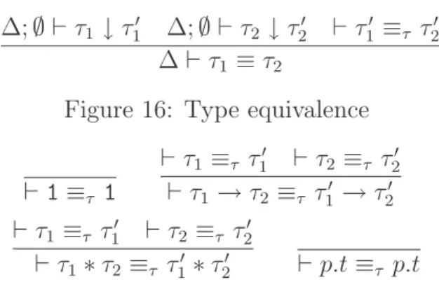
In this section, we develop a type expansion algorithm, which reduces types into canonical forms by unrolling type abbreviations. The purpose of the type expansion is to define type equality. Each type has a unique canonical form unless it does not contain dangling or cyclic references. Hence, once types are reduced into canonical forms we can judge their equality in a syntactic way.
Located types We first introduce canonical forms of types, named located
types, which are output from the type expansion. A located type consists
of simple located types and unit types. A simple located type is an abstract type, i.e.
Definition 5 A simple located type w.r.t. a program environment ∆ is a
type path p.t where p is in located form w.r.t. ∆ and either ∆ ` p 7→
(θ, ss . . . datatype t = c of τ . . . endi) or ∆` p 7→ (θ, sig . . . type t . . . endi)
holds.
For a type τ , typaths(τ ) denotes the set of type paths that τ contains. Precisely, typaths(τ ) =
typaths(τ1)∪ typaths(τ2) when τ = τ1 → τ2 or τ = τ1∗ τ2
{p.t} when τ = p.t
∅ when τ = 1
Then we define located types as follows.
Definition 6 A located type w.r.t. a program environment ∆ is a type τ
where each type τ0 in typaths(τ ) is a simple located type w.r.t. ∆.
4.1
Type expansion algorithm
We define the type expansion in Figure 15. The judgment ∆; Ω ` τ ↓ τ0 means that the expansion reduces the type τ into the type τ0 where Ω is locked w.r.t. the program environment ∆. We use Ω as a metavariable for sets of pairs (i, t) of an integer i and a type name t.
Observe that for any program environment ∆, lock Ω and type τ , proof search for ∆; Ω` τ ↓ is deterministic. We regard inference rules of the type
[tnlz-uni] −− ∆; Ω` 1 ↓ 1 [tnlz-arr] ∆; Ω` τ1 ↓ τ10 ∆; Ω` τ2 ↓ τ20 ∆; Ω` τ1 → τ2 ↓ τ10 → τ20 [tnlz-pair] ∆; Ω` τ1 ↓ τ10 ∆; Ω` τ2 ↓ τ20 ∆; Ω` τ1∗ τ2 ↓ τ10 ∗ τ20 [tnlz-dtyp] ∆` p ; p0 ∆` p0 7→ (θ, ss . . . datatype t = c of τ . . . endi) ∆; Ω` p.t ↓ p0.t [tnlz-atyp] ∆` p ; p0 ∆` p0 7→ (θ, ss . . . type t . . . endi) ∆; Ω` p.t ↓ p0.t [tnlz-abb] ∆` p ; p0 ∆` p0 7→ (θ, ss . . . type t = τ1. . . endi) − − −∆; Ω] (i, t) ` τ1 ↓ τ2 ∆; Ω` θ(τ2)↓ τ− − − ∆; Ω` p.t ↓ τ Figure 15: Type expansion
expansion as defining an algorithm which takes ∆, Ω and τ as input then either returns τ0 as output when the search succeeds in building a derivation tree for ∆; Ω ` τ ↓ τ0 or raises an error when the search fails. We prove termination of the proof search later in Proposition 7.
Let us examine each rule of the type expansion. The first three rules
[tnlz-uni], [tnlz-arr] and [tnlz-pair]are straightforward.
For a type type p.t, the expansion first reduces its prefix p into a located form p0 to determine the module that p refers to ( [tnlz-dtyp][tnlz-atyp][tnlz-abb]). When the module path expansion fails, then the type expansion fails too. Even though the module path expansion succeeds, the type expansion may fail, if p0 resolves to a functor; in that case the type path p0.t is dangling,
hence so is p.t. When the module path expansion succeeds in reducing p into
p0 and when p0 resolves to a structure or structure type, the type expansion continues. There are four possible cases:
1) The structure (type) does not contain a type component named t. In this case p.t is dangling.