THE RELATION BETWEEN INVESTORS GREEDINESS AND THE ASSET PRICE IN THE MEAN-VARIANCE MARKET

Journal of the Operations Research Society of Japan

Vol. 40, No. 4, December 1997

THE RELATION BETWEEN INVESTOR'S GREEDINESS A N D THE ASSET PRICE IN THE MEAN-VARIANCE MARKET

Hiroshi Konno Tokyo Institute of Technology

(Received December 5 , 1996; Revised March 27, 1997)

Abstract We will discuss the role of investor's "greediness", i.e., the investor's expected rate of return out of the investment, on the determination of the asset price in the multi-period portfolios owned by investors in the mean-variance capital market. We will derive the closed form of the equilibrium price vector and show that the average greediness of investors must be less than the expected rate of return of the market portfolio to guarantee the existence of a non-negative equilibrium price system. These results will be applied to the analysis of the "bubble" of the capital market and to the pricing of a new stock to be listed in the capital market.

1. Introduction

The purpose of this article is to analyze the relation between the equilibrium asset price and the greediness of investors, i.e., the expected rate of return of the portfolios owned by investors in the mean-variance capital market. Numerous papers concerning the equilibrium capital asset price have been published since the pioneering works of Sharpe [18], Lintner [g]

and Mossin [l l ] . For a surrey of these results, the readers are referred to [2,3,16,17]. Also readers can find more recent results in a series of papers by Nielsen [ 1 2 ~ 1 5 ] and Werner

[W

In a recent series of articles ([6], [7], [8]), the author derived explicit formulae of the equilibrium price vector of stocks in the capital market under several alternative assumptions on the behavior of investors.

The starting point of the research was Konno and Shirakawa[7], in which the authors assumed that the capital market satisfies the standard assumptions imposed in the CAPM type equilibrium analysis and derived a closed form of the equilibrium price vector in the mean-variance capital market where all risk averse investors choose their portfolios in view of the mean and variance of the rate of return of investment. In addition, we derived a necessary and sufficient condition for the existence of a unique non-negative equilibrium vector.

Also, Konno and Shirakawa [6] showed that a similar result holds in the mean-absolute deviation capital market where investors choose the absolute deviation instead of the vari- ance of the rate of return of investment as a measure of risk. Further, Konno and Suzuki [8] extended these results to a more general capital market in which the assumption about the homogeneity of investors is relaxed to allow different types of investors in the market.

The fundamental idea which enabled us to derive a "closed" form of the non-negative equilibrium vector is to interpret the rate of return of each asset as exogenously determined random varia,bles as in Mossinfll]. To be more precise,we consider that the distribution of the random variable

Rj,

representing the rate of return of unit investment into stock

Sj

is

580 PI. Konno

generated prior t o the transaction as a function of projected performance of the enterprise, interest rate and current stock price, etc..

This interpretation is different from the standard equilibrium approach in which the rate of return of assets is endogenously determined in the capital market as a function of the price of stocks. T h e analysis of the equilibrium price in this framework leads one t o a class of fixed point problems, for which it is very difficult, if not impossible to derive a closed form of the equilibrium price vector.

Another important assumption which is different from the traditional approach is t h a t short sale is not allowed in our model. This leads one t o an apparently more difficult opti- mization problem under inequality conditions. However, this assumption plays an essential role in deriving a necessary and sufficient condition for the existence of a unique non-negative equilibrium price vector, using a standard nonlinear programming methodology for handling non-negativity conditions.

T h e purpose of this article is two-folds. First, we will clarify the logical structure of our model in the framework of multi-stage decision problem and point out the importance of the "greediness", namely the expected rate of return of individual investors in the market. Second, we apply the results of equilibrium analysis to the pricing of a new stock t o be listed in the market.

In Section 2, we state the set of assumptions imposed in the subsequent analysis. In Section

3,

we extend the results of equilibrium analysis obtained in

[7]

to a multi-stage decision making environment. Section 4 will be devoted to the quantitative analysis of the effect of investor's expectation on the asset prices. We show that bubble can emerge when the investor's expectation grows beyond some bound.

In Section 5, we will present another potential application to the pricing of a new stock t o be listed in the market.

2. Assumptions

Let us assume that there exists n risky assets Sj(j = 1,

-

,

n ) and one riskless asset

So

in the capital market. Also, let us assume that there are m investors i = 1,

,

m with initial

0

endowments X: (xio, xyl,

.

,

X;-) where x O represents the units of asset

Sj

owned by i-th

i-J

investor at the beginning of the initial period. We will assume that all investors hold a non-negative amount of asset

Sj

( j = 0,1,

-

.

,

n):

0

X - -

>

0, j = 0 , 1 , - - . , n ;

i

= l , - - -

1] - m . (2.1)

At the beginning of each period t ( t = 1,2,

-

.

v ) , all investors sell their endowment X \ ' = ( XX

,

X ' ) in the market and purchase a new asset mix x1, = X:-,,

-

.

,

X:-) t o

maximize his/her utility U:, where U, is the function of the mean r and the variance v of the rate of return per period of the portfolio. Further we assume that the utility functions

U:

(r, v) satisfy the following conditions:

8 ~ j ( r , v)/&

>

0, 8 U h r , v)/&

<

0, _(2.2) for all i and t .

Let

R',

be the random variable representing the rate of return of stock

S,

during period

t.

We assume as usual that all investors share the same planning horizon and the complete knowledge of the the first two moments of the vector of random variable

R'

=

(R:,

-

.

,

R;) a t the beginning of period t.

Next we will assume that the capital market satisfies the following assumptions: Assumption 1. There is no friction (transaction costs and tax) associated with transaction.

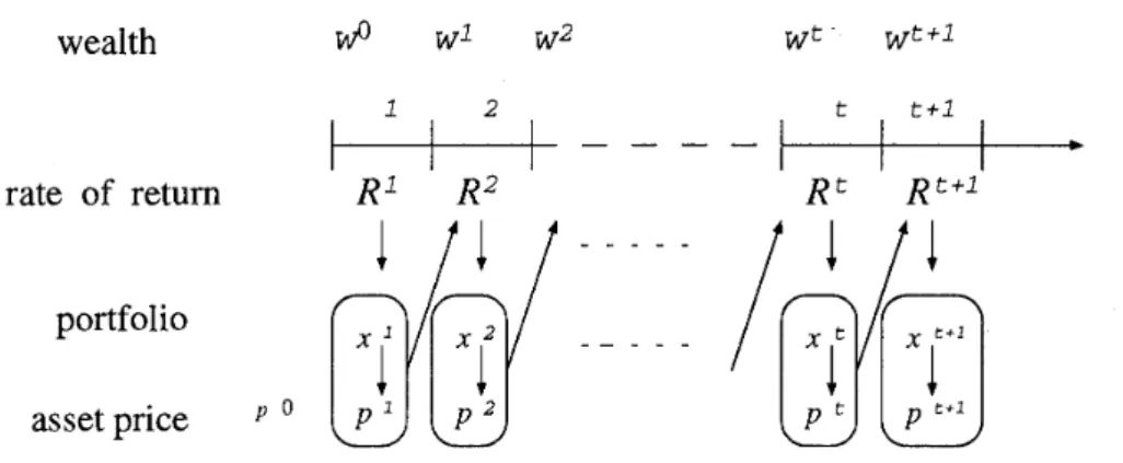
wealth WÂ w1 w2 wt - ^t+1 t+l

l*

- - - -

t

L

+

+

.

rate of return R1 R2 ~t ~ t + l portfolio asset price

Figure 3.1: Dynamic Structure of the Portfolio Selection

Assumption 3. Investors can borrow and/or lend riskless asset with the riskfree rate ro

without bound.

Assumption 4. Investors are not allowed to sell risky assets short.

Assumptions 1 3 are standard in the equilibrium analysis. T h e reason why we do not allow short sale is two-folds. First, as discussed in

[7],

this condition plays a crucial role in deriving a necessary and sufficient condition for the existence of a nonnegative equilibrium price vector. Second, the proportion of short sale is usually less than 10 percent in the Tokyo Stock Exchange. Also investors has t o clear the short sale within a limited length of time. Therefore, we can assume no short sale as a proxy of the capital market.

3. Price of Stocks in t h e Equilibrium Capital Market

Let p p = 0 , 1 ,

-

.

,

n ;

t

= 1 , 2 ,

. .

,

)

be the unit price of

Sj

during period

t

t o be determined in the market at the time of transaction. We will assume without loss of generality t h a t p^

the unit price of riskless asset

So

is unity for all

t .

Let X\, be the units of

Sj(j

= 0 , 1 , . , n )

to be owned by investor

i(i

= 1,

-

,

m ) during period

t

as a result of the transaction t o be exercised at the beginning of period

t .

Then the total value W: of the endowment X'' = ( x p

,

X:;',

.

)

,

:X: evaluated a t the

beginning of period

t

is given by n

j=o

Also the rate of return R(x') of the portfolio X: = (x:~, x : ~ ,

- -

,

xin) during period

t

is

given by

n

where

R;

is a random variable representing the rate of return of stock

Sj

during period

t .

We assume that the probability distribution of the random variables

R'

=

(R', R;,

,

R;)

is generated before the transaction via the past data such as Rs(s

<

t )

and p t l as well as through various economic projections (See Figure 3.1).

Then n t t t t E [ X ] =

'Z,

r&xi,/wi 7 j = O n n t t t t

V

E E

a } k ~ j ~ i ~ ~ k ~ i k / ( ~ ' ; ) ~ . j=1 k=l

where r: is the expected value of R x j = 0 , 1 ,

.,

n ) and a$ is the covariance of

R:

and

R;

(Note t h a t the rate of return Rh of the riskless asset

So

is a constant rh for all

t

so t h a t

582 H. Konno

The minimal variance of the rate of return of investment for a given value of the expected rate of return p can be calculated by solving the following convex quadratic programming problem:

minimize subject to

Let

X'.(/>) = ((^{P),

a),

-

) x ' . ~ ( P ) ) 7 (3.6)

be an optimal solution of (3.5) and let vxp) be the associated minimal variance. Then the mean-variance investor i whose utility function satisfies the condition (2.2) will choose p in such a way as t o maximize his/her utility Uxp, v:(p)). Let,

p\ = argmax Uxp, v',[p)).

P (3.7)

Let us introduce a canonical quadratic programming problem:

n n

minimize

E ~ Z ~ Z ~

and assume that this problem has a unique optimal solution zt = (2:) z\.

-

,

4."

It is easy

to show (See[7]) that ~ { ( p ) , the minimal variance associated with problem (3.5)) is given by

:=l

Therefore, p\ of (3.7) is independent of p'. Also we can assume without loss of generality that

t t

Pi

>

To) (3.10)

since each investor can achieve ( r , v) = (rh, 0) by investing his/her total wealth into riskless assets.

Theorem 3.1 Optimal asset mix (xJl,

- -

,

xjn) of the i-th investor is given by the following formula:

t t t t t t .

p - X . . _{. I t 3} = (p, - ro)wiz,, j = l , - + , n . (3.11) Proof

This theorem states that all investors hold a portfolio of risky assets proportional t o the vector zt =

-

,

4).

Therefore the vector

n

"This condition is satisfied if for example the following conditions hold. (i) rj > 7-0, j = l , - - - , n,

defines t h e market portfolio associated wit h period t

.

To achieve a n equilibrium, the following market clearance condition

i=1 i = l

has to be satisfied. From (3.13) and (3.11), we obtain the relation

m m m

- r t ) & .

0 2 . 1 (3.14)

i=1 i=1 1=1

Using t h e equation (3.1) and the assumption p* = 1, we obtain a system of equation t o be satisfied by the equilibrium price vector, namely

m m n m

Theorem 3.2 A necessary and sufficient condition for the system of equation (3.15) to have a unique solution is given by

in which case the equilibrium price pi is given by

m m

p'J = E ( p ; - r : ) x : i l m l - m:) Ex;;',

j

= 1 , - . - , n .

i=1 Proof

Let

and let a = (al,

-

,

b = (bl,

-

.

,

bn)T and pt = (pi,

- ,

pi)T

where the superscript

"T" stands for the transposition of vectors. Then the equation (3.15) can be represented as follows:

(I - = bao.

This equation has a unique solution if and only if a T b

#

1 (See [4]). It easy t o check that condition is equivalent to (3.16). Also, it is easy to check that the unique solution is given by

Hence we have (3.17). D

Let us introduce a n additional assumption, which is satisfied for t = 1 by (2.1).

m

Assumption 5. E ( p ; - r 3 x t i 1

2

0 for all t. i=l

Note t h a t p\ - r; >_ 0 for all z and

t .

Therefore this assumption holds if x:;l 0 for all

i.

If

there are many "disturbing" investors with large p\ and very negative x:il, then Assumption

5 may not be valid.^

m

^he sum of riskless asset in the market Mt-i =

Ex;'

is usually significantly larger than individual

2x1

584 H. Konno

Corollary 3.3 The price of risky assets are non-negative if and only if m*

<

1 under Assumption

5.

Proof The result follows from (3.17) since ( i pi

2

r' for all i and

t

by (3.10).

(ii)

4

2

0 for all

t

since z t is an optimal solution of (3.8)

( )

E

=

E

=

-

=

y>yj

>

0 by noting (2.1).

We see from this equation that the equilibrium price p^, is

(i) an increasing function of the amount x g l of the riskless asset owned by investors, (ii) a decreasing function of the rate of return r; of riskless asset,

(iii) an increasing function of p:, the expected rate of return of i-th investor.

Let us note that similar results can be obtained under alternative assumptions on the be- havior of investors. In fact, we obtained explicit formula of the equilibrium price vector under alternative measures of risk, from which we can derive the same conclusions as above. (See [7,

81

for details).

4. Role of Investor's Expectation

It has been proved in Theorem 3.1 that x^,(i = 1,

. .

,

m; j = 1, .

,

n ) satisfies the relation

t t t t t t

xi, = ( p i - ro)wizj/pj. (4.1)

Let

4-

b e the fraction of security j held by investor i after the transaction a t the beginning of period t. Then by (4.1), we have

m m

This means that the Q;:. is independent of j, which in turn implies that

t t -

o". = a . J = l

22 2 7 , . . . , n ,

for all

t

1. Let us define two constants:

n

i=l

where yj's are defined in (3.12). The constant r'^/ is the expected rate of return of the market portfolio yt during period

t.

Also p h is the average of the expected rate of return of all investors in the market where the weight is chosen as the proportion of risky assets owned by individual investors. The constant may be called the "market greediness".

Theorem 4.1 Let t

>

2. Then the condition m:

<

1 holds if and only if in which case Proof By (3.16) we have m n m0 =

E

- r;)

E

4

= (PM - ro)

E

4

i=1 j=1 j=1 Also by (3.12), we have

J=l J=l

Further z\ satisfies the relation

n n J=1 j=1 Hence n ₁

G;Â

= t J=1 rM - rk

.

Therefore

so that m:

<

1 if and only if p\

<

rb,

in which case p: >_ 0 for all j since x g l is always 2=1

m m

nonnegative. Substituting (4.8) into (3.17) yields (4.7) by noting that

E x \ ,

=

E x : ,

for

i= l i=1

all

t

>

1.

It is now easy t o compute the total value of risky assets

l$

a t the beginning of period

t ( 2

2).

Corollary 4.2 Let

Mt

be the total amount of riskless asset in the capital market during period

t .

Then

Proof

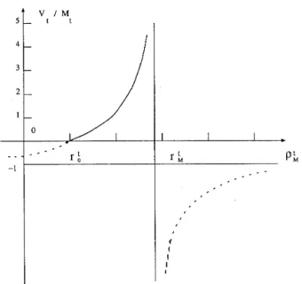
We see from Figure 4.1 that the total value V; of risky assets is zero when = rk. It is an increasing function of the market greediness p& and it grows t o infinity as p^ approaches

r\. When p\ exceeds r L , then the price of stock becomes negative which means t o the collapse of t h e market. Let us define the "temperature" of the capital market

T 7"

which represents the proportion of the risky assets relative to tot a1 assets outstanding in the capital market. By (4.9)) we have an alternative representation of K f :

PL

- r;

K t = (4.11)

rM - r Q

This means t h a t is an indicator of the closeness of p^ to r\i,. If is close t o 1, then the market is overheated and is in danger.

T h e market temperature is a macro-economic constant which can be recovered from the market data. Unfortunately however, it is not easy to identify

Mt

and V; in the capital market. One possible surrogate variable for the total amount of the riskless asset

Mt

would

H. Konno

Figure 4.1: Total Value of Risky Assets as a Function to the Market Greediness be the total amount of outstanding Government bonds. Also, the total value of risky assets

V, may be represented by the sum of the total value of stocks and bonds.

5. Pricing of a New Stock to be Listed in the Market

Let us consider the pricing of a new stock

Sn+1

to be listed in the market. Let us assume that the amount of riskless asset Vo, the rate of return of riskless asset ro, and the market greediness P M remain constant before and after the listing. Given the starting price p L 1 ,

we may be able to calculate the distribution of the random variable Rn+l(pE+l) representing the rate of return of Sn+1.

Then we can calculate the expected rate of return rn+l E rn+l(pitl) and the covariance coefficient i7jn+l i 7 j n + l ( p ~ + l ) ( j = 1,

,

n

+

1). A new market portfolio (z;,

,

_{z;, zZtl)}

will be calculated by solving an n

+

1-dimensional quadratic programming problem:

subject to ( r j - ro)zj = 1

j=l

l

.q

>

0, j = 1 , - - - , n , n

+

l.

Thus we can calculate the price p L l of the stock

Snt1

after the listing by using the formula (4.7) :

* - PM - r0

( r h

- r ~ ) A f ~ z ; + l / ~ n + i j = 1 , - - - , n

+

1,

^

W

rb

- P M (5.2)

where s n + ~ is the unit of stock n

+

1 to be released, z x j = 1, , n , n

+

1) is an optimal solution of (5.1). Also the expected rate of return r h of the new market portfolio is given

r& =

X

rjz;

+

rn+lz;+l.

j=l

(5.3)

The calculated p h may not be equal to p¡Â . The adequate price of

Sntl

is therefore

0

the value of p n + ~ for which p^, = p,,.,.,.

We will assume that both S and

S

are positive definite. Let 2 = ( ^ l , - . * , z n ) T

W = ( ^ i , - * - , ~ , ~ n + l ) ~

p = (rl - r0.r; - r o , - - - , r n - ro)-

1

f i = (rl - r 0 7 ~ 2 - r o , - . . , r n -ro)rn+i - T O )

J

T h e canonical quadratic program corresponding to n assets and n

+

1 assets are given by minimize z t S z subject t o g z = 1 z > o (5.6) minimize W SW subject t o fiTw = 1 w > o -

Let us introduce quadratic programs by dropping the nonnegativity constraint from (5.6)

and (5.7):

minimize z t S z

subject t o $ z = 1

minimize W

SW

subject t o

f i

= 1

T h e optimal solutions of these problems are given by

2 = s - l p / ~ T s - l ~

A s s u m p t i o n 6. 2

>

o , W

>

o.

Under this assumption, 2 and W of (5.10) and (5.11) give optimal solutions of (5.6) and (5.7), respectively.

T h e o r e m 5.1 Let ( p l ,

-

, p n ) be the equilibrium price of assets

Sj

( j

= 1 ,

-

.,

n ) in the market. Also let (p:,

,

p:+l) be the new equilibrium price after the introduction of Sn+l. Then

Proof _Let U = ( p i ~ l , . . . ipnsn)T and V* = (p;si, . - - iP>n7P:+l~n+l)T. By noting the

relation (5.10), (5.11) and (4.17), we have U = a S 1 p

v * = "S-lA*

or equivalently

Let W = (v',

-

.

,

v')T. Then SW

+

U V ^ ~ =

a^<

from which we obtain

T --l

Let us consider a special case in which

rh

= r~ and

fi

S

fi

= a l p . Then 6 = a

so that we have

n

Note that Rn+1 is a function of Therefore /tn+l, 0 and 0 ~ + 1 , ~ + \ are functions of p¡+l

The equilibrium price may be obtained by solving the equation

n

Therefore, we will be able to calculate the appropriate value of pn+l if the explicit relation between pn+l and /tn+l, qn+1 (j = I , - .

,

rz

+

1) can be estimated.

Acknowledgements. Part of this research was supported by Grant-in-Aid for Scientific Research of the Ministry of Education, Science and Culture, Grant No. ( A ) ( l ) 08305002. Also, the author is grateful to the generous support of the Dai-ich Mutual Life Insurance, Co. and the Toyo Trust and Banking, Co..

References

F.

Black, Capital Market Equilibrium with Restricted Borrowing,

J.

of Business, 45 (1972), 444-454

G. M. Constantinides and A. G. Malliaris, Portfolio Theory, Chapter 1 of Handbook of

OR&MS, Vol 9 (Jarrow et al. eds.), 1995.

Elton, E.

J.

and Gruber M., Modern Portfolio Theory and Investment Analysis, 4th Edition, John Wiley & Sons, 1991

F.

R. Gantmacher, The Theory of Matrices, Chelsea Publishing Co., New York, 1964

0.

D. Hart, On the Existence of Equilibrium in a Security Model, J. of Economic Theory, 9 (1974), 293-311

H.

Konno, and

H.

Shirakawa, Equilibrium Relations in the Mean- Absolute Deviation Capital Market, Financial Engineering and the Japanese Markets, 1 (1994), 21-35. H. Konno, and H. Shirakawa, Existence of a Nonnegative Equilibrium Price Vector in the Mean-Variance Capital Market, Mathematical Finance, 5 (1995)) 233-245.

H. Konno and

K.

Suzuki, Equilibria in the Capital Market with Non-Homogeneous Investors, Japan

J.

of Industrial and Applied Mathematics, 13 (1996), 369-383.

J.

Lintner, The Valuation of Risk Assets and the Selection of Risky Investments in Portfolio Choice, Review of Economics and Statistics, 47 (1965), 13-37

589

[l01 D.

G.

Luenberger, Introduction to Linear and Nonlinear Programming, 2nd Edition, John Wiley & Sons, 1984

1 l]

J.

Mossin, Equilibrium in Capital Asset Market, Econometrica 34 (1966), 768-783 [l21 L.T.Nielsen, Portfolio Selection in t h e Mean-Variance Model: A Note,

J .

of Finance,

42 (1987)) 1371-1376

[l31 L.T. Nielsen, Asset Market Equilibrium with Short Selling, Review of Economic Studies, 56 (1989)) 467-474

[l41 L.T. Nielsen, Equilibrium in CAPM without a Riskless Asset, Review of Economic Studies, 57 (1990), 315-324

[l51 L.T. Nielsen, Existence of Equilibrium in CAPM,

J.

of Economic Theory, 52 (1990)) 223-231

[l61

R.

Roll, A Critique of the Asset Pricing Theory's Tests; Part I : On Past and Potential Testability of t h e Theory, J. of Financial Economics, 4 (1977)) 129-176

[l71 S. A. Ross, T h e Current Status of t h e Capital Asset Pricing Model (CAPM),

J.

of Finance, 33 (1978)) 885-901

[ l ]

W.F.

Sharpe, Capital Asset Prices : A Theory of Market Equilibrium under Condition of Risk, J. of Finance, 19 (1964)) 425-442

[l 91 J

.

Werner

,

Arbitrage and the Existence of Competitive Equilibrium, Econometrica, 55 (1987), 1403-1418

Hiroshi KONNO

Department of Industrial Engineering and Management Tokyo Institute of Technology

Meguro-ku, Tokyo, 152, Japan (E-mail: konno0rne.titech.ac.j p)