2009, Vol. 52, No. 1, 46-57
AN EOQ MODEL FOR DETERIORATION ITEMS UNDER TRADE CREDIT POLICY IN A SUPPLY CHAIN SYSTEM
Jui-Jung Liao Kun-Jen Chung
Chihlee Institute of Technology Chung Yuan Christian University
(Received September 14, 2006; Revised October 28, 2008)
Abstract This paper attempts to determine economic order quantity for deteriorating items under the conditions of permissible delay in payments, in which the supplier offers the retailer a permissible delay period and the retailer in turn provides a maximal trade credit period to their customers in a supply chain system. A theorem is developed to determine the optimal ordering policies for the retailer under above conditions. These results help the retailer’s decision makers to determine accurately the optimal cost. A numerical example demonstrates the applicability of the proposed method. Moreover, sensitivity analysis of the optimal solution with respect to major parameters is carried out. Finally, the results in this paper generalize some already published results.
Keywords: Inventory, trade credit, deterioration, permissible delay in payments
1. Introduction
A supply chain (Chopra and Meindl [3]) consists of all stages involved, directly or indirectly, in fulfilling a customer request. The supply chain not only includes the manufacturers and suppliers, but also transporters, warehouses, retailers and customers themselves. So, the supply chain management (Levi et al. [23]) is a set of approaches utilized to efficiently integrate them so that merchandiser is produced and distributed at the right quantities, to the right location and at the right time, in order to minimize systemwide costs.
Goyal [11] is the first to establish an economic order quantity model under the condition of permissible delay in payments. He assumes that the supplier would offer the retailer a fixed delay period and the retailer could sell the goods and accumulate revenue and earn interest within the trade credit period. Goyal [11] implicitly assumes that the customer would pay for the items as soon as the items are received from the retailer. That is, Goyal [11] assumed that the supplier would offer the retailer a delay period but the retailer would not offer the trade credit period to customers. In most business transactions, this assumption is debatable. Huang [15] defines this situation as one level of trade credit. Huang [13] extends Goyal [11] to provide a fixed trade credit period M between the supplier and the retailer and a maximal trade credit period N (M > N ) between the retailer and the customer. Basically, the inventory model of Goyal [11] is a supply chain of two stages (the supplier and the retailer). Huang [13] generalizes Goyal [11] to the supply chain of three stages [the supplier, the retailer and customers]. Huang [15] names the above situation two levels of trade credit.
On the other hand, Ghare and Schrader [10] are pioneers to develop an EOQ model by negative exponential distribution which investigation assumes that the instantaneous deterioration rate is constant. Combining Ghare and Schrader [10] and Goyal [11], numerous
be found in Jaggi and Aggrawal [16], Aggarwal and Jaggi [1], Arcelus et al. [2], Chu et al. [4], Chung and Liao [8, 9], Chung and Huang [7], Liao [18, 19], Tsao and Shreen [25] and their references.
All the above papers mentioned do not consider deteriorating items and two levels of trade credit together. So, the main purpose of this paper is to extend Huang [13] into the inventory model under two levels of trade credit to more match a real life situation.
2. Model Formulation
The following notations are used throughout the whole paper: Notations:
A: ordering cost per order p: unit selling price per item c: unit purchasing price per item.
D: demand rate per year
Ie: interest earned per $ per year
Ik: interest charged per $ in stock per year by the supplier
M : the retailer’s trade credit period offered by supplier in years
N : the maximal trade credit period for customers offered by retailer in years h: unit stock holding cost per unit per year excluding interest charges
T : the cycle time in years
T V C(T ): the annual total relevant cost T∗: the optimal cycle time of T V C(T )
In addition, the following assumptions are used throughout: Assumptions:
1. Demand rate is known and constant. 2. The shortages are not allowed.
3. Time period is infinite and replenishment lead time is zero.
4. The distribution of time to deterioration of the items follows exponential distribution with parameter θ (constant rate of deterioration).
5. Ie ≤ Ik, M ≥ N and p ≥ c.
6. A supplier allows a fixed period, M , to settle the account. During this fixed period no interest is changed by the supplier but beyond this period, interest Ik is charged by the
supplier under the terms and conditions agreed upon. The account is settled completely either at the end of the credit period or at the end of the cycle.
7. A retailer allows a maximal trade credit period N for customers to settle the account. If a customer buys one item from the retailer at time t belonging to (0,N ], then the customer will have a trade credit period N − t and make the payment at time N. Furthermore, the retailer can accumulate revenue and earn interest after the customer pays for the amount of purchasing cost until the end of the trade credit period offered by the supplier. That is, the retailer can accumulate revenue and earn interest during the period N to M with rate Ie under the condition of trade credit.
Recently, Assumption (7) is rather prevalent. It has been adopted in a lot of papers such as Huang [13–15], Teng and Chang [24], Liao [20], Ho et al. [12], Ouyang et al. [21], Jaggi et al. [17] and their references.
Let Q(t) denote the on−hand inventory level at time t, which is depleted by the effects of demand and deterioration, then the differential equation which describes the instantaneous
states of Q(t) over (0, T ) is given as:
dQ(t)
dt + θ Q(t) =−D, 0≤ t ≤ T (2.1)
then, with boundary condition Q(T ) = 0. The solution of equation (2.1) is given by
Q(t) = D θ (e
θ(T−t)− 1), 0≤ t ≤ T (2.2)
Noting that Q(0) = Q, then quantity ordered each replenishment cycle is
Q = D
θ(e
θT − 1) (2.3)
Furthermore, the total relevant cost function per cycle is the sum of the ordering cost, inventory holding cost, cost of deteriorated units and interest payable on stock held beyond the permissible period, less the interest earned during the period of (N, M ). From now on, the individual cost is evaluated before they are grouped together.
1. Annual ordering cost= A T
2. Annual inventory holding cost(excluding interest charges) = h T ∫ T 0 Q(t)dt = hD θ2T(e θT − θT − 1)
3. Annual cost of deteriorated units= c(Q−DT )T = cDθT(eθT − θT − 1)
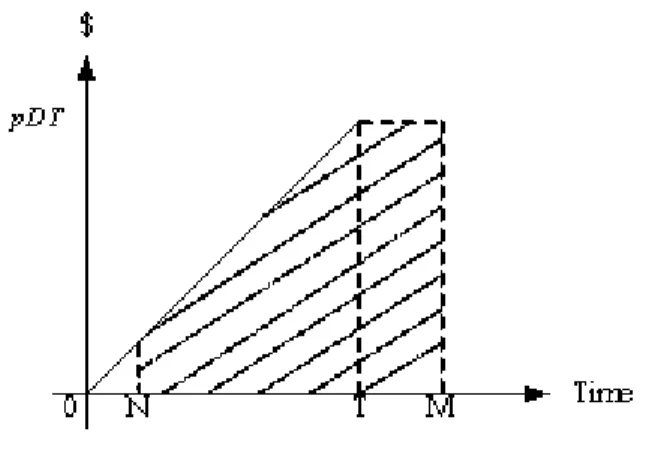
4. Regarding interests charged and earned, we have the following three cases to discuss: Case(I): T ≥ M, shown in Figure 1.
In this case, the sales revenue is utilized to earn interest Ie during the period of (N, M ).
When the account is settled, the item still in inventory has to financed with annual rate Ik.
Therefore, the annual interest payable is
cIk ∫T M Q(t)dt T = cIkD θ2T (e θ(T−M)− θ(T − M) − 1)
From Figure 1, it implied that the retailer sells products and deposits the revenue into an account during period (0, N ], but getting money at time N. Therefore, sales revenue, pDN , is continuous accumulated from period (N, M ) and the interest earned of this part is pIe,
multiplied by the area of N M Y Z. In addition, the sales revenue from period (N, M ) is continuous accumulated, so the interest earned of this part is pIe multiplied by the area of
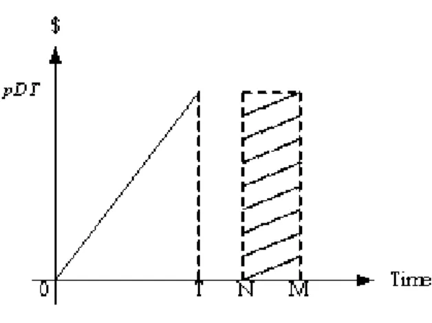
XY Z. Combining the above argument, the annual interest earned is pIe ∫ M N Dtdt T = pIeD(M2 − N2) 2T = pIeD(M + N )(M − N) 2T Case(II):N ≤ T < M, shown in Figure 2.
In this case, all the sales revenue is utilized to earn interest with annual rate Ie during
the period of (N, M ) and pays no interest for the items kept in stock. Therefore, the annual interest payable is 0, and the annual interest earned is
pIe[ ∫T N D tdt + DT (M− T )] T = pIeD 2T [2M T − N 2− T2]
Figure 1: The total accumulation of interest earned when M ≤ T
Figure 2: The total accumulation of interest earned when N ≤ T ≤ M
Case(III):T ≤ N, shown in Figure 3.
In this case, all the sales revenue is utilized to earn interest Ie during the period of
(N, M ) and pays no interest for the items kept in stock as well. Therefore, the annual interest payable is 0, and the annual interest earned is
pIe ∫M
N DT dt
T = pIeD(M − N)
Combining the above arguments, we obtain that the annual total relevant cost per unit time is given by T V C(T ) = T V C1(T ) if M < T T V C2(T ) if N < T ≤ M T V C3(T ) if 0 < T ≤ N (2.4) where T V C1(T ) = A T + D(cθ + h) θ2T (e θT−θT −1)+cIkD θ2T (e θ(T−M)−θ(T −M)−1)−pIeD(M2− N2) 2T (2.5) T V C2(T ) = A T + D(cθ + h) θ2T (e θT − θT − 1) − pIeD 2T (2M T − N 2− T2) (2.6)
Figure 3: The total accumulation of interest earned when T ≤ N and T V C3(T ) = A T + D(cθ + h) θ2T (e θT − θT − 1) − pI eD(M − N) (2.7)
For convenience to discuss, we extend the domain of T V Ci(T ) (i = 1, 2, 3) and treat the
domain of T V Ci(T ) (i = 1, 2, 3) as (0,∞). Then, equation (2.5) yields
T V C1′(T ) = −A T2 + D(cθ + h) θ2T2 (θT e θT − eθT + 1) +cIkD θ2T2(θT e θ(T−M)− eθ(T−M)+ 1− θM) + pIeD(M2− N2) 2T2 (2.8) After rearrangement, T V C1′(T ) = 1 θ2T2 { −Aθ2+ D(cθ + h)(θT eθT − eθT + 1) +cIkD(θT eθ(T−M)− eθ(T−M)+ 1− θM) + pIeD(M2− N2)θ2 2 } = 1 θ2T2f (T ) where f (T ) = −Aθ2+ D(cθ + h)(θT eθT − eθT + 1) +cIkD(θT eθ(T−M)− eθ(T−M)+ 1− θM) + pIeD(M2− N2)θ2 2
Since f′(T ) = Dθ2T [(cθ + h)eθT + cIkeθ(T−M)] > 0 , so f (T ) is increasing on T > 0 . Let
T1∗ denote the root of T V C1′(T ) = 0. Since lim
T→∞f (T ) =∞ > 0, the following results hold.
(i) If f (M ) < 0, then T1∗ > M .
(ii) If f (M )≥ 0, then T1∗ = M .
On the other hand, equations (2.6) and (2.7) yield
T V C2′(T ) =−A T2 + D(cθ + h) θ2T2 (θT e θT − eθT + 1)− pIeD 2T2 (N 2− T2), (2.9)
T V C2′′(T ) = 2A T3 + 2D(cθ + h) θ2T3 [ eθT ( 1− θT + 1 2θ 2T2 ) − 1]+pIeDN 2 T3 > 2A T3 + 2D(cθ + h) θ2T3 [ eθT · e−θT − 1]+pIeDN 2 T3 = 2A T3 + pIeDN2 T3 > 0, (2.10) T V C3′(T ) =−A T2 + D(cθ + h) θ2T2 (θT e θT − eθT + 1), (2.11) and T V C3′′(T ) = 2A T3 + 2D(cθ + h) θ2T3 [ eθT ( 1− θT +θ 2T2 2 ) − 1 ] > 2A T3 + 2D(cθ + h) θ2T3 [ eθT · e−θT − 1] = 2A T3 > 0 (2.12)
Therefore, T V C2(T ) and T V C3(T ) is convex on (0,∞),respectively. Since T V C1(M ) =
T V C2(M ) and T V C2(N ) = T V C3(N ), T V C(T ) is continuous and well-defined. 3. Decision Rule Of The Optimal Cycle Time T∗
Consider the following equations:
T V Ci′(T ) = 0 (i = 1, 2, 3) (3.1)
If the root of equation (3.1) exists, then it is unique. Let Ti∗ (i = 1, 2, 3) denote the root of equation (3.1). Further, equations (2.8), (2.9) and (2.11) yield that
T V C1′(M ) = T V C2′(M ) = − A M2 + D(cθ + h) θ2M2 (θM e θM − eθM + 1) +pIeD(M 2− N2) 2M2 (3.2) and T V C2′(N ) = T V C3′(N ) = − A N2 + D(cθ + h) θ2N2 (θN e θN − eθN + 1) (3.3)
Since T V C2(T ) is convex on T > 0 which implies that T V C2′(M ) > T V C2′(N ). For convenience, let
∆1 =− A M2 + D(cθ + h) θ2M2 (θM e θM − eθM + 1) + pIeD(M2− N2) 2M2 (3.4) and ∆2 =− A N2 + D(cθ + h) θ2N2 (θN e θN − eθN + 1) (3.5)
∆1 < 0 if and only if T V C1′(M ) < 0 if and only if T1∗ > M . ∆1 < 0 if and only if T V C2′(M ) < 0 if and only if T2∗ > M . ∆2 < 0 if and only if T V C2′(N ) < 0 if and only if T2∗ > N . ∆2 < 0 if and only if T V C3′(N ) < 0 if and only if T3∗ > N .
Furthermore, if ∆1 ≥ 0, then T V C1(T ) is increasing on [M,∞).The above arguments lead to the following results.
Theorem 1
1. If ∆1 < 0, then T V C(T∗) = T V C(T1∗). Hence T∗ is T1∗.
2. If ∆2 > 0, then T V C(T∗) = T V C(T3∗). Hence T∗ is T3∗.
3. If ∆1 ≥ 0 and ∆2 < 0, then T V C(T∗) = T V C(T2∗). Hence T∗ is T2∗. Proof:
1. If ∆1 < 0, then ∆2 < 0 which implies that T1∗ > M , T2∗ > M , T2∗ > N and T3∗ > N , respectively. Furthermore, T V C(T ) has the minimum value at T = N when T ≤ N,
T V C(T ) has the minimum value at T = M when N ≤ T ≤ M and T V C(T ) has the
minimum value at T = T1∗ when T ≥ M. Since T V C3(N ) = T V C2(N ) > T V C2(M ) and T V C2(M ) = T V C1(M ) > T V C1(T1∗), T V C(T ) has the minimum value at T1∗ for
T > 0. Hence, we conclude that T V C(T∗) = T V C(T1∗). Consequently, T∗ is T1∗.
2. If ∆2 > 0, then ∆1 > 0 which implies that T2∗ < M , T2∗ < N , T3∗ < N and T V C1(T ) is increasing on [M,∞). Furthermore, T V C(T ) has the minimum value at T = T3∗ when
T ≤ N, T V C(T ) has the minimum value at T = N when N ≤ T ≤ M and T V C(T )
has the minimum value at T = M when T ≥ M. Since T V C3(T3∗) < T V C3(N ) =
T V C2(N ) < T V C2(M ) and T V C2(M ) = T V C1(M ), T V C(T ) has the minimum value at T3∗ for T > 0. Hence, we conclude that T V C(T∗) = T V C(T3∗). Consequently, T∗ is T3∗.
3. If ∆1 ≥ 0 and ∆2 < 0 which implies that T1∗ < M , T2∗ < M , T2∗ > N and T3∗ > N . Furthermore, T V C(T ) has the minimum value at T = N when T ≤ N, T V C(T ) has the minimum value at T = T2∗ when N ≤ T ≤ M and T V C(T ) has the minimum value at T = M when T ≥ M. Since T V C3(N ) = T V C2(N ) > T V C2(T2∗) and
T V C2(T2∗) < T V C2(M ) = T V C3(M ). Hence, we conclude that T V C(T∗) = T V C(T2∗). Consequently, T∗ is T2∗.
Combining the above arguments, we have completed the proof. 4. Numerical Examples
In order to illustrate the above solution procedure, let us consider an inventory system with the following data:
A = $200/order, h = $5/unit/year, c = $60/unit/year, p = $70/unit/year, Ik = 20%,
Ie= 12%, θ = 0.01, M = 0.3year and N = 0.2year.
Example 1:When D = 400 units/year, then ∆1 =−166.6464 < 0 and ∆2 =−3878.5 < 0. Using Theorem 1(1), we get T∗ = T1∗ = 0.307, the optimal order quantity is Q∗ = 122.9887 and T V C(T∗) = T V C(T1∗) = 722.4254.
Example 2:When D = 1800 units/year, then ∆1 = 7027.9 > 0 and ∆2 = 46.7250 > 0. Using Theorem 1(2), we get T∗ = T3∗ = 0.1991, the optimal order quantity is Q∗ = 358.7370 and T V C(T∗) = T V C(T3∗) = 496.6506.
Example 3:When D = 500 units/year, then ∆1 = 347.2476 > 0 and ∆2 =−3591.8 < 0. Using Theorem 1(3), we get T∗ = T2∗ = 0.2847, the optimal order quantity is Q∗ = 142.5528 and T V C(T∗) = T V C(T2∗) = 734.3698.
minimum total relevant cost per unit time T V C(T∗) of the following data:
A = $200/order, h = $5/unit/year, c = $60/unit/year, p = $70/unit/year, Ik = 20%,
Ie = 12%, D = 1000 units/year, θ = 0.01, M = 0.3year and N = 0.2year. The sensitivity
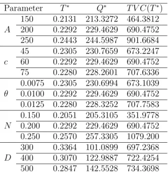
analysis is performed by changing each of the parameters by −25% and +25%, taking one parameter at a time and keeping the remaining parameters unchanged. The results are summary in Table 1.
Table 1: Sensitivity analysis
Parameter T∗ Q∗ T V C(T∗) 150 0.2131 213.3272 464.3812 A 200 0.2292 229.4629 690.4752 250 0.2443 244.5987 901.6684 45 0.2305 230.7659 673.2247 c 60 0.2292 229.4629 690.4752 75 0.2280 228.2601 707.6336 0.0075 0.2305 230.6994 673.1039 θ 0.0100 0.2292 229.4629 690.4752 0.0125 0.2280 228.3252 707.7583 0.150 0.2051 205.3105 351.9778 N 0.200 0.2292 229.4629 690.4752 0.250 0.2570 257.3305 1079.200 300 0.3364 101.0899 697.2368 D 400 0.3070 122.9887 722.4254 500 0.2847 142.5528 734.3698
Based on the results of Table 1, the following observation can be made.
1. A higher value of ordering cost A results in higher values of T∗, Q∗ and T V C(T∗). Additionally, we find that T V C(T∗) are highly sensitive to changes in A.
2. A higher value of retailer’s trade credit N results in higher values of T∗, Q∗ and
T V C(T∗). Additionally, we find that T∗, Q∗ and T V C(T∗) are highly sensitive to the changes in N .
3. A higher value of purchasing price c results in a higher value of T V C(T∗), but lower values of T∗ and Q∗. It indicates that if we increase the purchasing price, then the optimal length of ordering cycle and the optimal ordering quantity will be decreased. 4. A higher value of deteriorating rate θ results in a higher value of T V C(T∗), but lower
values of T∗ and Q∗. It tells us that when the deteriorating rate increases, the optimal length of ordering cycle and the optimal ordering quantity will be decreased.
5. A higher value of demand rate D results in higher values of T V C(T∗) and Q∗, but a lower value of T∗.
5. Special Cases
In this section, there are the following cases to occur: (i) Shah’ model
When N = 0 and p = c, we have
T V C(T ) = { T V C1S(T ) if M ≤ T, T V CS 2(T ) if M > T. (5.1)
where T V C1S(T ) = A T + D(cθ + h) θ2T (e θT − θT − 1) +cIkD θ2T (e θ(T−M)− θ(T − M) − 1) − cIeDM2 2T (5.2) and T V C2S(T ) = A T + D(cθ + h) θ2T (e θT − θT − 1) −cIeD 2T (2M T − T 2) (5.3) Equations (5.2) and (5.3) are consistent with equations (13) and (10) in Shah [22], respec-tively. Furthermore, we let
∆ = D(cθ + h)(θM e θM − eθM + 1) θ2M2 + cIeD 2 − A M2 Then, we have the following results.
Corollary 2 1. T V C1S(T ) is convex on [M,∞). 2. T V CS 2(T ) is convex on (0,∞). 3. T V C(T ) is convex on (0,∞). Corollary 3 1. If ∆ > 0, then T∗ is T2∗. 2. If ∆ < 0, then T∗ is T3∗. 3. If ∆ = 0, then T∗ = T2∗ = T3∗ = M .
The results of Corollaries 2 and 3 have been discussed in Chung [6]. (ii) Goyal’s model
When θ → 0+, N = 0 and p = c, we have
T V C(T ) = { T V C1(T ) if M ≤ T, T V C2(T ) if M > T. (5.4) where T V C1(T ) = A T + DT h 2 + cIkD(T − M)2 2T − cIeDM2 2T (5.5) and T V C2(T ) = A T + DT h 2 − cIeD(2M T − T2) 2T (5.6)
Equations (5.5), (5.6) are consistent with equations (1) and (4) in Goyal [11] ,respectively. Furthermore, we let
∆∗ = DM
2(h + cI
e)− 2A
2 Then, we have the following results.
Corollary 4
1. If ∆∗ > 0, then T∗ is T2∗. 2. If ∆∗ < 0, then T∗ is T3∗.
(iii) Huang’s model
When θ → 0+ and p = c, we have
T V C(T ) = T V C1∗(T ) if M < T T V C2∗(T ) if N < T ≤ M T V C3∗(T ) if 0 < T ≤ N (5.7) where T V C1∗(T ) = A T + DT h 2 + cIkD(T − M)2 2T − cIeD(M2− N2) 2T (5.8) T V C2∗(T ) = A T + DT h 2 − cIeD(2M T − N2− T2) 2T (5.9) and T V C3∗(T ) = A T + DT h 2 − cIeD(M− N) (5.10) Equations (5.8), (5.9) and (5.10) are consistent with equations (2), (3) and (4) in Huang [13], respectively. Furthermore, we let
∆1 =−2A + DM2(h + cIe)− cDN2Ie
and
∆2 =−2A + DN2h Then, we have the following results.
Corollary 5
1. If ∆1 < 0, then T∗ is T1∗.
2. If ∆2 > 0, then T∗ is T3∗.
3. If ∆1 > 0 and ∆2 < 0, then T∗ is T2∗.
The results of Corollary 5 have been discussed in Huang [13]. 6. Summary
This paper considers a supply chain system consisting of one supplier, one retailer and multiple customers to explore the optimal retailer’s replenishment decisions under the con-ditions of permissible delay in payments, in which the supplier offers the retailer a fixed delay period and the retailer in turn provides a maximal trade credit period to their cus-tomers. Theorem 1 gives the solution procedure to find T∗. Numerical examples are given to illustrate Theorem 1. In addition, sensitivity analysis represents the following results: first,
T∗, Q∗ and T V C(T∗) increase with increase in the values of parameters A and N . Second,
T∗ and Q∗ decrease while T V C(T∗) increases with increase in the values of parameters c and θ. Third, T∗ decreases while Q∗ and T V C(T∗) increase with increase in the value of parameter D. Additionally, although the optimal cycle time cannot be expressed in a closed form, it can be obtained through the use of the Intermediate Value Theorem [26]. More-over, if N = 0 and p = c, Shah [22] can be treated as a special case of this paper. Finally, if the deterioration is ignored, Equations (2.4) are reduced to Goyal [11] and Huang [13], respectively.
References
[1] S.P. Aggarwal and C.K. Jaggi: Ordering policies of deteriorating items under per-missible delay in payments. Journal of the Operational Research Society, 46 (1995), 658–662.
[2] F.J. Arcelus, N.H. Shah, and G. Srinivasan: Retailer’s pricing, credit and inventory policies for deteriorating items in response to temporary price/credit incentives.
Inter-national Journal of Production Economics, 81-82 (2003), 153–162.
[3] S. Chopra and P. Meindl: Supply Chain Management: Strategy, Planning, and
Opera-tion (Prentice-Hall Inc, 2001).
[4] P. Chu, K.J. Chung, and S.P. Lan: Economic order quantity of deteriorating items under permissible delay in payments. Computers & Operations Research, 25 (1998), 817–824.
[5] K.J. Chung: A theorem on the determination of economic order quantity under condi-tions of permissible delay in payments. Computers & Operacondi-tions Research, 25 (1998), 49–52.
[6] K.J. Chung: The inventory replenishment policy for deteriratingf items under permis-sible delay in payments. Opsearch, 37 (2000), 267–281.
[7] K.J. Chung and T.S. Huang: The optimal retailer’s ordering policies for deteriorating items with limited storage capacity under trade credit financing. International Journal
of Production Economics, 106 (2007), 127–145.
[8] K.J. Chung and J.J. Liao: Lot-sizing decisions under trade credit depending on the ordering quantity. Computers & Operations Research, 31 (2004), 909–928.
[9] K.J. Chung and J.J. Liao: The optimal ordering policy in a DCF analysis for deteri-orating items when trade credit depends on the order quantity. International Journal
of Production Economics, 100 (2006), 116–130.
[10] P.M. Ghare and G.F. Schrader: A model for exponentially decaying inventories. Journal
of Industrial Engineering, 14 (1963), 238–243.
[11] S.K. Goyal: Economic order quantity under conditions of permissible delay in payment.
Journal of the Operational Research Society, 36 (1985), 335–338.
[12] C.H. Ho, L.Y. Ouyang, and C.H. Su: Optimal pricing, shipment and payment policy for an integrated supplier-buyer inventory model with two-part trade credit. European
Journal of Operational Research, 187 (2008), 496–510.
[13] Y.F. Huang: Optimal retailer’s ordering policies in the EOQ model under trade credit financing. Journal of the Operational Research Society, 54 (2003), 1011–1016.
[14] Y.F. Huang: An inventory model under two levels of trade credit and limited storage space derived without derivatives. Applied Mathematical Modelling, 30 (2006), 418–436. [15] Y.F. Huang: Optimal retailer’s replenishment decisions in the EPQ model under two levels of trade credit policy. European Journal of Operational Research, 176 (2007), 1577–1591.
[16] C.K. Jaggi and S.P. Aggarwal: Credit financing in economic ordering policies of dete-riorating items. International Journal of Production Economics, 34 (1994), 151–155. [17] C.K. Jaggi, S.K. Goyal, and S.K. Goel: Retailer’s optimal replenishment decisions
with credit-linked demand under permissible delay in payments. European Journal of
Operational Research, 190 (2008), 130–135.
[18] J.J. Liao: On an EPQ model for deteriorating items under permissible delay in pay-ments. Applied Mathematical Modelling, 31 (2007), 393–403.
to ordering quantity. Applied Mathematical Modelling, 31 (2007), 1690–1699.
[20] J.J. Liao: An EOQ model with noninstantaneous receipt and exponentially deteriorat-ing items under two-level trade credit. International Journal of Production Economics, 113 (2008), 852–861.
[21] L.Y. Ouyang, C.K. Ho, and C.H. Su: Optimal strategy for an integrated system with variable production rate when the freight rate and trade credit are both linked to the order quantity. International Journal of Production Economics, 115 (2008), 151–162. [22] N.H.Shah: A lot-size model for exponentially decaying inventory when delay in
pay-ments is permissible. Cahiers du CERO, 35 (1993), 115–123.
[23] D. Simchi-Levi, P. Kaminsky, and E. Simchi-Levi: Designing and Managing the Supply
Chain (The McGraw-Hill Book Companies, Inc, 2000).
[24] J.T. Teng and C.T. Chang: Optimal manufacturer’s replenishment policies in the EPQ model under two levels of trade credit policy. European Journal of Operational Research, 195 (2009), 358–363.
[25] Y.C. Tsao and G.J. Shreen: Dynamic pricing, promotion and replenishment policies for a deteriorating item under permissible delay in payments. Computers & Operations
Research, 35 (2008), 3562–3580.
[26] D. Varberg, E.J. Purcell, and S.E. Rigdon: Calculus (Pearson Education, Inc, 2007). Jui-Jung Liao
Department of Business Administration Chihlee Institute of Technology,
Taiwan, ROC.