Spectrogram consistency and its application to phase reconstruction

全文

(1)Vol.2009-MUS-81 No.8 2009/7/30 IPSJ SIG Technical Report. exactly ensured, one should at least look for outputs which are “as consistent as possible”. This is in particular the case when trying to resynthesize a signal from a modified magnitude STFT spectrogram, for which there is in general no phase such that their combination is consistent. Carefully studying the structure of complex STFT spectrograms and quantifying the consistency of a set of complex numbers is thus a crucial issue. In this article, we derive explicit consistency constraints for STFT spectrograms as the kernel of a simple linear operator in the complex time-frequency domain with coefficients depending on the window length, the frame shift and the analysis and synthesis windows used to build the spectrogram or which the spectrogram is assumed to have been obtained from. The norm of the image of a set of complex numbers by this linear operator defines a numerical consistency criterion, which can for example be used as a prior distribution on complex spectrograms when performing separation tasks in the complex time-frequency domain, or, as we shall investigate here, as an objective function on the phase when trying to recover the most coherent phase for a given magnitude spectrogram. We will first derive consistency constraints for STFT spectrograms, then explain how to define a numerical consistency criterion based on them, and finally introduce an algorithm for phase reconstruction based on the optimization of an objective function derived from the consistency criterion and show how it can be used to develop a flexible real-time time-scale modification algorithm.. Spectrogram consistency and its application to phase reconstruction Jonathan Le Roux,†1 Hirokazu Kameoka,†1 Nobutaka Ono†2 and Shigeki Sagayama†2 In this article, we derive the constraints which a set of complex numbers must verify to be a consistent STFT spectrogram, i.e., to be the STFT spectrogram of an actual real-valued signal, and describe how they lead to an objective function measuring the consistency of a set of complex numbers as a spectrogram. We then present a flexible phase reconstruction algorithm based on a local approximation of the consistency constraints and derive a real-time time-scale modification algorithm.. 1. Introduction Many acoustical signal processing techniques, developed for a wide range of applications such as source separation [7, 11–13], noise canceling [2], time-scale and pitch-scale modifications or more generally audio modification [6], involve a processing of the time-frequency representation of a signal obtained by the short-time Fourier transform (STFT). However, as the STFT representation is usually obtained from overlapping frames of a waveform, it is redundant and characterized by a particular structure. Starting from a set of complex numbers in the complex time-frequency domain, it is thus not guaranteed whether there exists a signal in the time domain whose STFT is equal to that set of complex numbers. Therefore, to avoid irrealistic solutions, any processing performed on STFT spectrograms should ensure that its outputs are “consistent spectrograms”, i.e., that they all are the STFT of some time-domain signal, or, when dealing with magnitude or power spectrograms, that there exist phases which can be coupled with the ouput magnitude spectrograms to give consistent spectrograms. If consistency cannot be. 2. Characterization of consistent STFT spectrograms 2.1 Perfect reconstruction constraints on the window functions Let (x(t))t∈Z be a digital signal. We review here the conditions for perfect reconstruction of the signal through STFT and inverse STFT [1, 4]. Let N be the window length, R the window shift, w the analysis window function and s the synthesis window function. We suppose that w and s are zero outside the interval 0 ≤ t ≤ N − 1. We assume that the window length N is an integer multiple of the shift R, and we note Q = N/R. We shall denote by θ = (w, s, N, R) the set of all parameters related to analysis and synthesis. It can be shown [4] that there is perfect reconstruction through the inverse STFT under the following necessary conditions: Q−1 ∑ 1= w(t − qR)s(t − qR), ∀t. (1). †1 NTT コミュニケーション科学基礎研究所 NTT Communication Science Laboratories †2 東京大学大学院情報理工学系研究科 Graduate School of Information Science and Technology, The University of Tokyo. q=0. 1. c 2009 Information Processing Society of Japan ⃝.

(2) Vol.2009-MUS-81 No.8 2009/7/30 IPSJ SIG Technical Report. By introducing the coefficients k+qR 1 ∑ (θ) αq,p = w(k)s(k + qR)e−j2πp N − δp δq , N. 2.2 Consistency operator Let (Hm,n )0≤m≤M −1,0≤n≤N −1 be a set of complex numbers, where m will correspond to the frame index and n to the frequency band index, and w and s be analysis and synthesis windows verifying the perfect reconstruction conditions (1) for a frame shift R. STFTw will denote the STFT with analysis window w, and iSTFTs the inverse STFT with synthesis window s. When not indicated, we will assume that we use w and s respectively. As we are interested here in spectrograms corresponding to real-valued signals, we shall assume in the following that N = 2P and that all the sets of complex numbers considered are “conjugate symmetric”, i.e., ∀n ∈ [[1; P − 1]], H(m, P + n) = H(m, P − n) and the elements at frequency band indices 0 and P are realvalued. These sets form an R-vector subspace of CM ×N , denoted by S . STFT spectrograms obtained from real-valued signals are examples of such sets, but the point to be made in this paper is that not all such sets can be obtained as STFT spectrograms of real-valued signals. For the set H to be a consistent STFT spectrogram, it needs to be the STFT spectrogram of a signal x(t), which by perfect reconstruction can be none other than the result of the inverse STFT of the set (Hm,n ). A necessary and sufficient condition for H to be a consistent spectrogram is thus for it to be equal to the STFT of its inverse STFT. The point here is that, for a given window length N and a given frame shift R, the operation iSTFTs ◦STFTw from the space of real-valued signals of length T = (M −1)R+N to itself is the identity, while STFTw ◦ iSTFTs from S to itself is not. Altogether, the set of consistent spectrograms can be described as the kernel of the R-linear operator from S to itself defined by Fw,s (H) = (STFTw ◦ iSTFTs − I M N )(H), (2) where I L denotes the L×L identity matrix. We shall refer to this operator as the “consistency operator”, and write F instead of Fw,s when there is no ambiguity. 2.3 Derivation of explicit consistency constraints We can derive consistency constraints for STFT spectrograms in the timefrequency domain by explicitly stating that a consistent spectrogram H must be in the kernel of F. A simple computation leads to the following expression for the image of H by F: Q−1 N −1 ∑ ∑ ′ k+qR n 1 ∑ F(H)m,n = w(k)e−j2πk N s(k + qR) Hm−q,n′ ej2πn N − Hm,n . N ′ k. q=−(Q−1). (4). k. where −(N − 1) ≤ p ≤ N − 1 and δi is the Kronecker delta (δ0 = 1 and δi = 0 for i ̸= 0), and stating that F(H)m,n must be equal to 0 for all m and n, we can obtain the consistency constraints we are looking for, summarized in the following Proposition. For analysis and synthesis windows w and s verifying the perfect reconstruction conditions (1) for a frame shift R, a set of complex numbers H ∈ S is a consistent spectrogram if and only if, ∀m ∈ [[0, M − 1]], ∀n ∈ [[0, N − 1]], Q−1 N −1 ∑ ∑ qR (θ) F(H)m,n = ej2π N n αq,n−n′ Hm−q,n′ = 0, (5) n′ =0 q=−(Q−1) (θ). where the coefficients α are defined by (4). The interesting point in the above relation is that we characterized the consistency of a set of complex numbers directly in the time-frequency domain, without having to make apparent the connection with a certain time domain signal. 3. Numerical consistency criterion 3.1 Relaxing the constraints Equation (5) represents the relation between a set of complex numbers and the STFT of its inverse STFT, as its left member is F(H). Instead of enforcing consistency through the “hard” constraints (5), which may be difficult to handle, these can be relaxed by introducing any vector norm of F(H): this indeed leads to a numerical criterion which can be used to quantify how far a set of complex numbers is from being consistent. We can for example consider in particular the L2 norm of F(H), as we will show later on that this special choice leads to a criterion which is related to that used by Griffin and Lim to derive their iterative STFT algorithm [4]. This defines a consistency criterion I(H) = ||F(H)||2 as follows: ∑

(3)

(4)

(5) F(H)m,n

(6) 2 . I(H) = (6) m,n. 3.2 Consistency as a penalty function We can think of using numeral consistency criterions such as (6) as penalty functions, for example when working on source separation or spectrogram modification algorithms in the complex time-frequency domain. In such situations. n =0. (3). 2. c 2009 Information Processing Society of Japan ⃝.

(7) Vol.2009-MUS-81 No.8 2009/7/30 IPSJ SIG Technical Report. where one attempts to estimate complex spectrograms following certain properties from an input signal, ensuring that the estimated sets of complex numbers are consistent spectrograms is both likely to lead to better, because more consistent and thus more meaningful, results, and to ease the optimization process by reducing the dimension of the problem, as it will tend to discard solutions which are not coherent. We shall however leave these issues to forthcoming papers and investigate here the use of the consistency criterion introduced above to define an objective function on phase when the magnitude is fixed, as described in the next section.. ˜ (k) ) I(φ. d(x(k+1) , A) x ˆ(k+1). x ˆ(k). jφ(k+1). Ae. Aejφ. (k). 4. Phase reconstruction for a modified STFT spectrogram We consider here the application of the consistency criterion (6) to develop an algorithm for reconstructing the most consistent phase given a modified magnitude STFT spectrogram. The iterative STFT algorithm introduced by Griffin and Lim [4] is the reference for such algorithms. Its principle is to find the consistent STFT spectrogram with magnitude closest to a given modified magnitude spectrogram. On the other hand, the algorithm we propose looks for a phase such that the spectrogram obtained by associating it with that magnitude spectrogram is as consistent as possible. Although conceptually close to the iterative algorithm, a crucial difference is that it operates directly in the time-frequency domain. 4.1 Objective function for phase reconstruction problems In the problem of phase reconstruction, we are given a set of real non-negative numbers Am,n which are supposedly the amplitude part of an STFT spectrogram, for example obtained through modifications of the power spectrum of a sound. The goal is to estimate the phase ϕm,n to adjoin to A such that Am,n ejϕm,n is as close as possible to be a consistent STFT spectrogram. This amounts to minimizing the consistency criterion I w.r.t. the phase ϕ, with the amplitude A given, defining the following objective function:

(8) 2 ∑

(9)

(10) ∑ qR

(11) (θ) ˜ ej2π N n αq,p I(ϕ) = Am−q,n−p ejϕm−q,n−p

(12) , (7)

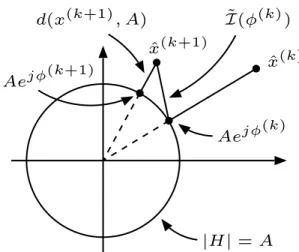
(13). |H| = A Fig. 1 Illustration of the iterative STFT algorithm and the relation between the objective function I˜ and the squared distance d(x, A). (k+1). (k+1). x ˆ(k+1) the STFT of x(k+1) , and ϕm,n the phase of x ˆ(k+1) , ϕm,n = ∠ˆ x(k+1) . They showed that this procedure estimates a real-valued signal x which minimizes (at least locally) the squared distance

(14) 2 ∑

(15)

(16)

(17) d(x, A) = x|m,n − Am,n

(18) , (8)

(19) |ˆ m,n. i.e., the squared error between the magnitude of the STFT x ˆ of x, and the magnitude spectrogram A. As can be seen in Fig. 1, we shall note that the objective function I˜ measures a slightly different quantity from the squared distance (8), but that the iterative STFT algorithm also converges to a minimum of (7). Indeed, both quantities become equivalent near convergence, as one can ˜ (k) ) ≤ d(x(k) , A) [4]. However, the objective funcshow that d(x(k+1) , A) ≤ I(ϕ ˜ tion I we introduced has the advantages to be explicit and defined directly in the time-frequency domain, and in its general version (6) not to be limited to phase reconstruction problems with fixed magnitude. 4.2 Direct optimization of I˜ The iterative STFT algorithm, as mentioned above, can be used to minimize ˜ However, this can be considered as an indirect minimization, and it is worth I. looking at a direct minimization of I˜ through classical optimization methods.. m,n p,q s.t. |n−p|∈[[0,N −1]]. In [4], Griffin and Lim presented the iterative STFT algorithm, which consists (k) in iteratively updating the phase ϕm,n at step k by replacing it with the phase of the STFT of its inverse STFT while keeping the magnitude A. The algorithm (k) is illustrated in Fig. 1, where x(k+1) denotes the inverse STFT of Am,n ejϕm,n ,. 3. c 2009 Information Processing Society of Japan ⃝.

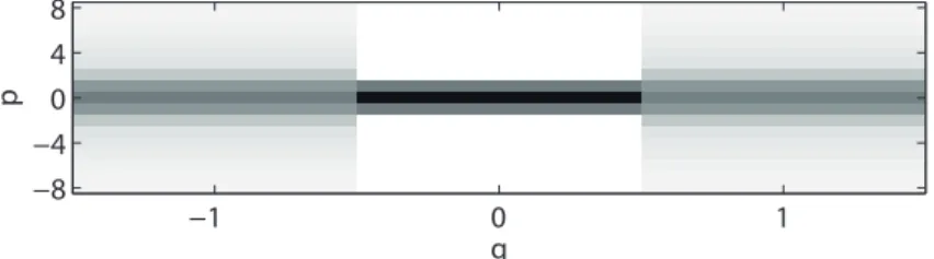
(20) Vol.2009-MUS-81 No.8 2009/7/30 IPSJ SIG Technical Report. p. This will indeed provide us with the freedom to modify/approximate the objective function on one hand, and to select how each bin will be dealt with on the other. One could for example decide not to update the phase for certain bins which are considered reliable. Further in this direction, one could try to reconstruct bins which have been discarded by a binary mask from the bins which have been determined as reliable by minimizing the consistency criterion (6) with respect to both the magnitude and phase of those bins while keeping others fixed. Finally, one could also imagine introducing weights depending on frequency to emphasize stronger consistency in certain frequency regions based on perceptual criteria, or on magnitude to give more importance to the reduction of inconsistency around bins with large magnitude. The bin selection presented in Section 4.4 is a discrete version of this last idea. 4.3 Approximate objective function and phase coherence Here, we will make the following two approximations. We will first neglect the influence of ϕm,n in all the terms F(H)m′ ,n′ other than F(H)m,n , which (θ) is the one where it is multiplied by α0,0 . The motivation behind this first ap(θ) proximation is that the coefficient α0,0 dominates over the other coefficients. By assuming the other phase terms fixed, we will then update each bin’s phase ϕm,n (θ) so that α0,0 Am,n ejϕm,n is in opposite direction with the terms coming from the neighboring bins, while keeping its amplitude Am,n fixed. This corresponds to (θ) performing a coordinate descent [14]. More precisely, as α0,0 = 1/Q − 1 < 0, the update for bin (m, n) is ( ) ∑ qR (θ) ej2π N n αq,p ϕm,n ← ∠ Hm−q,n−p . (9). 8 4 0 −4 −8 −1. 0 q. 1. (θ). Fig. 2 Magnitude of the central coefficients αq,p for N = 512, R = 256, a Hanning analysis window and a rectangular synthesis window.. would be involved if using terms. The update becomes: ) ( all the∑ qR (θ) Hm−q,n−p , ϕm,n ← ∠ ej2π N n αq,p. (10). (p,q)̸=(0,0) s.t. |p|≤l. where frequency indices are understood modulo N . For l = 2 and a 50 % overlap, for example, we only consider 5 × 3 coefficients. 4.4 Taking advantage of sparseness As evoked above, using a direct optimization of the objective function I˜ enables us to select which bins to update. This can be the key to deal with problems where only a part of the spectrogram has to have its phase reconstructed, but it can also in general be used to lower the computational cost. Indeed, we can use the sparseness of the acoustic signal to limit the updates to bins with a significant amplitude, or progressively decrease the amplitude threshold above which the bins are updated, starting with the most significant bins and refining afterwards. This idea can be related to the peak picking techniques in [5, 6]. 4.5 Exact optimization through an auxiliary function method We note that the objective function (7) can be minimized based on an auxiliary function method. Let (Gm,n m′ ,n′ ) be the matrix representation of F. We then have ∑ m,n F(H)m,n = m′ ,n′ Gm,n m′ ,n′ Hm′ ,n′ . If we introduce auxiliary variables Z m′ ,n′ such ∑ m,n m,n that ∀m, n, m′ ,n∑ ′ Z m′ ,n′ = 0, then for any such Z and for any δm′ ,n′ > 0 such m,n that for all m, n, m′ ,n′ δm′ ,n′ = 1, we can show that

(21) 2 ∑ 1

(22)

(23) m,n m,n jϕm′ ,n′

(24) ||F(H)||2 ≤ (11)

(25) . m,n

(26) Z m′ ,n′ − Gm′ ,n′ Am′ ,n′ e δm′ ,n′ ′ ′. (p,q)̸=(0,0) s.t. |n−p|∈[[0,N −1]] (θ). Second, noticing that most of the weight in the coefficients αq,p is actually concentrated near (0, 0), as can be seen in Fig. 2 for a window length N = 512 and a frame shift R = 256, with a Hanning analysis window and a rectangular synthesis window, we can further approximate the update equations (9) by using only (2l + 1) × (2Q − 1) central coefficients instead of the total N × (2Q − 1), where l ≪ N . This approximation is motivated by the importance of local phase coherences, in particular the so-called “horizontal” and “vertical” coherences, to obtain a perceptually good reconstructed signal, and can be considered close to phase-locking techniques [5, 6, 10]. This approximation enables us to compute directly the update of each bin through the summation of a few terms, instead of the whole convolution which. m,n,m ,n. Minimizing the auxiliary function in the right-hand term first w.r.t. Z then w.r.t. ϕ leads to the following update(equation for ϕ: ) ϕm,n ← Arg am,n Hm,n − (F H F(H))m,n , (12). 4. c 2009 Information Processing Society of Japan ⃝.

(27) Vol.2009-MUS-81 No.8 2009/7/30 IPSJ SIG Technical Report. ∑ m′ ,n′ 2 m′ ,n′ where am,n = depends on the choice of δ. As δ is of m′ ,n′ |Gm,n | /δm,n very large dimension, it is preferable to set it in such a way that a can be m,n computed ∑ directly without explicitely computing δ. If we consider δm ′ ,n′ = m,n q m,n q |Gm′ ,n′ | / m′ ,n′ |Gm′ ,n′ | , where q > 0 is a tunable exponent, we get ∑ (θ) ∑ (θ) am,n = |αm′ ,n′ |2−q |αm′ ,n′ |q = a. (13) m′ ,n′. and introduce artifacts of their own [6]. These artifacts have been shown to be mainly connected to phase incoherences, and special care must thus be taken when estimating the phases in the modified signal’s STFT spectrogram. The iterative STFT algorithm of Griffin and Lim has been proposed as a way to correct such phase incoherences, although the computational cost and the slow speed of convergence have been obstacles to its adoption in commercial applications. The algorithm we introduced is a flexible alternative to iterative STFT, and by an active use of sparseness and the reduction of the number of multiplications involved at each step, should lead to a lower computational cost. 4.6.2 Sliding-block analysis for real-time processing Inspired by an idea in [9], we derive a real-time optimization scheme for the objective function introduced above based on a sliding-block analysis. The spectrogram is not processed all at once, but progressively from left to right, making it possible to change the parameters while sound is being played. The waveform to be time-scaled is read N samples at a time and with an average frame shift of f R where f is the time-scale multiplication factor. The phase updates described above are performed only on a sliding block of b frames. Frames exiting the sliding block are then used to resynthesize the output signal, with a frame shift R, leading to a signal whose length is 1/f times the length of the original signal. This way of building intermediate frames of the spectrogram is arguably more reliable than interpolating neighboring spectrogram frames and leads to an initial estimate of the phase which can be used as a starting point for both the iterative STFT and the proposed method. 4.6.3 Experimental evaluation We implemented the proposed method and the iterative STFT algorithm and compared their convergence speed on the time-scale modification of the first 23 s of Chopin’s Nocturne No. 2. The time-scale modification factor was set to 0.7, the frame length to 1024 and the frame shift to 512, for a final length of approximately (θ) 32 s. We used a 5 × 3 approximation of the coefficients αq,p for our algorithm. We ran our algorithm in two different experimental conditions, one where all the bins are updated at each iteration, and the other relying on sparseness, where at iteration k, only bins whose amplitude is larger than Ae−Bk are updated. Here, we used A = 1 and B = 0.005, which were determined experimentally. The objective function I(H) is used as a measure of convergence, and represented in decibels, with the initial value as a reference. A comparison of the speed of convergence in terms of the decrease of I(H) w.r.t.. m′ ,n′. Intuitively, a acts as a learning weight in Eq. (12): the larger a, the slower ϕ will move from its current value. As convergence is guaranteed anyway, we should thus look ∑ for a as small as possible, which is the case for q = 1, where we have a = ( |α|)2 . We then have ( ) ϕ ← Arg aH − F H F(H) . (14) It is interesting to note the link with Griffin and Lim’s update, which can be written with our notations as ( ) ϕ ← Arg H + F(H) , (15) In the special case where the windows w and s are equal (for example with the sine window), then F H = F and one can see that F H F(H) = −F(H). The only difference is then the a factor. We haven’t been able so far to find a setting for δ which would lead to a equal to or close to 1, and noticed through experiments that, due to that factor, Griffin and Lim’s update was faster than the auxiliary approach one in terms of the decrease of inconsistency per iteration. We plan to investigate this issue in the future as well. 4.6 Time-scale modification 4.6.1 Need for an efficient frequency-domain algorithm Many methods for time-scale and pitch-scale modification of acoustic signals have been proposed, and the interest on this subject intensified in recent years with the increase in the commercial application of such techniques. So far, most commercial implementations rely on time-domain methods, usually variations on Synchronous Overlap and Add (SOLA) or Pitch Synchronous Overlap and Add (PSOLA) techniques [8]. Their advantages are a low computational cost and good quality results for small modification factors (smaller than ±20 % or ±30 %) and monophonic sounds. For larger factors, polyphonic sounds or non-pitched signals, however, the quality of the results drops severely. On the other hand, frequency-domain methods, such as the phase vocoder [3], are not limited to such constraints, but they involve a much higher computational cost. 5. c 2009 Information Processing Society of Japan ⃝.

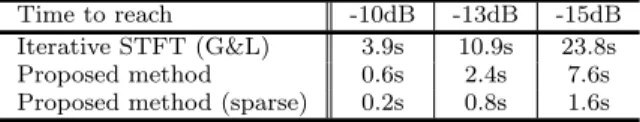
(28) Vol.2009-MUS-81 No.8 2009/7/30 IPSJ SIG Technical Report. STFT spectrograms, and explained how it could be used to introduce penalty functions in the complex time-frequency domain and to define an objective function on phase when working in the time-frequency magnitude or power domain. We developed a flexible phase reconstruction algorithm which can take advantage of the sparseness of the input signal and can take into account regions where phase is reliable. We applied this algorithm for time-scale modification, and explained how to perform a real-time processing based on a sliding-block analysis.. Inconsistency (dB). 0 Iterative STFT Proposed method Proposed method (sparse). −5 −10 −15 0. 50. 100 Nb. of iterations. 150. 200. Acknowledgments. Fig. 3 Comparison of the evolution of the inconsistency measure I(H) w.r.t. the number of iterations for the iterative STFT algorithm and the proposed method.. The authors would like to thank Dr. Emmanuel Vincent for fruitful discussions. References. Table 1 Computation time (s) required to reach a certain decrease of the inconsistency measure I Time to reach Iterative STFT (G&L) Proposed method Proposed method (sparse). -10dB 3.9s 0.6s 0.2s. -13dB 10.9s 2.4s 0.8s. 1) Allen, J.B. and Rabiner, L.R.: A unified approach to short-time Fourier analysis, Proc. of the IEEE, Vol.65, No.11, pp.1558–1564 (1977). 2) Boll, S.: Suppression of Acoustic Noise in Speech Using Spectral Subtraction, IEEE Trans. ASSP, Vol.27, pp.113–120 (1979). 3) Dolson, M.: The phase vocoder: A tutorial, Computer Music Journal, Vol.10, No.4, pp.14–27 (1986). 4) Griffin, D.W. and Lim, J.S.: Signal Estimation from Modified Short-Time Fourier Transform, IEEE Trans. ASSP, Vol.32, No.2, pp.236–243 (1984). 5) Karrer, T., Lee, E. and Borchers, J.: PhaVoRIT: A Phase Vocoder for Real-Time Interactive Time-Stretching, Proc. ICMC, pp.708–715 (2006). 6) Laroche, J. and Dolson, M.: Improved Phase Vocoder Time-Scale Modification of Audio, IEEE Trans. SAP, Vol.7, No.3, pp.323–332 (1999). 7) Le Roux, J., Kameoka, H., Ono, N., de Cheveign´e, A. and Sagayama, S.: Single Channel Speech and Background Segregation through Harmonic-Temporal Clustering, Proc. WASPAA, pp.279–282 (2007). 8) Moulines, E. and Laroche, J.: Non-Parametric Techniques for Pitch-Scale and Time-Scale Modification of Speech, Speech Comm., Vol.16, pp.175–206 (1995). 9) Ono, N., Miyamoto, K., Kameoka, H. and Sagayama, S.: A Real-time Equalizer of Harmonic and Percussive Components in Music Signals, Proc. ISMIR, pp.139–144 (2008). 10) Puckette, M.S.: Phase-locked vocoder, Proc. WASPAA (1995). 11) Schmidt, M.N. and Mørup, M.: Nonnegative Matrix Factor 2-D Deconvolution for blind Single Channel Source Separation, Proc. ICA, pp.700–707 (2006). 12) Smaragdis, P.: Discovering Auditory Objects Through Non-Negativity Constraints, Proc. SAPA (2004). 13) Virtanen, T.: Monaural Sound Source Separation by Nonnegative Matrix Factorization With Temporal Continuity and Sparseness Criteria, IEEE Trans. ASLP, Vol.15, No.3, pp.1066–1074 (2007). 14) Zangwill, W.I.: Nonlinear Programming: A Unified Approach, Prentice Hall (1969).. -15dB 23.8s 7.6s 1.6s. the number of iterations (or, equivalently, the block size) is shown in Fig. 3. One can see that, although our algorithm is based on an approximation of the original objective function I(H), it outperforms the iterative STFT algorithm in terms of speed of convergence as the number of iterations required to reach a given decrease of inconsistency. We also compared the computation times of the three methods, measuring only the time required by the phase reconstruction part of the algorithm as the other parts are identical. With our implementations, for 200 iterations, the iterative STFT algorithm took 29.1 s, our method with full updates 24.2 s, and our method using sparseness 2.1 s. Looking at the amount of time required to reach a certain decrease in inconsistency illustrates how our method, by combining speed of convergence and lower computational cost, leads to a much shorter computational time than iterative STFT, as illustrated in Table 1 for the experimental conditions described above. In terms of flexibility, speed of convergence and computation time, our algorithm thus outperforms the iterative STFT algorithm. 5. Conclusion We introduced a general framework to assess for the consistency of complex. 6. c 2009 Information Processing Society of Japan ⃝.

(29)