第 巻 第 号 抜 刷
年 月 発 行
Basic Research Spending,
Applied Research Subsidy, and Growth Cycles
Basic Research Spending,
Applied Research Subsidy, and Growth Cycles
Kunihiko Konishi
*abstract
This study constructs a variety-expansion growth model that integrates basic research to analytically examine growth cycles. We show that the equilibrium path can exhibit two-period cycles through the interplay between applied and basic research. In addition, we explore the effects of change in basic research spending and applied research subsidy. Under certain conditions, the steady-state growth rate increases when basic research spending or applied research subsidy increases. However, the effects on the possibility of cyclical instability differ by applied and basic research policies. An increase in basic research spending reduces the possibility of cyclical instability, while an increase in applied research subsidy raises the possibility of cyclical instability.
.Introduction
It is widely known that the long-run growth of developed countries is fluctuating, and a number of studies have investigated the existence of endogenous
cycles from various perspectives using R&D-based models.) However, few studies
focus on the linkage between basic research and economic fluctuation. Empirical
*Faculty of Economics, Matsuyama University, − Bunkyo-cho, Matsuyama-shi, Ehime − , JAPAN
)See Shleifer( ), Gale( ), Deissenberg and Nyssen( ), Francois and Shi( ), Freeman et al.( ), Matsuyama( ), Francois and Lloyd-Ellis( , , ), and Wälde( ).
studies argue that basic research contributes to the development of the economy
(Griliches, ; Jaffe, ; Mansfield, ; Cohen et al., ) and the
theoretical implications of basic research policy have been considered through
various macroeconomic viewpoints.) Thus, it is important to consider the existence
of endogenous cycles within a R&D-based model that integrates basic research. The present study theoretically examines the role of basic research in growth
cycles. To do this, we incorporate basic research into a variety-expansion model
following Grossman and Helpman( ). In our model, basic research generates
ideas, whereas applied research commercializes them by transforming them into
blueprints for new varieties of consumption goods. These two research sectors
interplay through knowledge spillovers. Further, we assume that basic research is
publicly funded−and thus, that the government can control the level of basic
research. According to Table in Gersbach et al.( ), which summarizes
data from a selection of countries, the average share of basic research that was
financed by governments and higher educational institutions was . % ; that is,
basic research is mainly funded by the government and conducted at universities or
other public research institutions. In addition, on an average, . % of applied
research was financed by business enterprises and private non-profit institutions ; that is, applied research is primarily performed by private firms motivated by their own benefits.
We show that the equilibrium path can exhibit two-period cycles through the
interplay between applied and basic research. The key driving force that gives rise
to cycles is the knowledge spillovers between applied and basic research. In our
)Cozzi and Galli( , , ), Chu et al.( ), and Chu and Furukawa( ) analyze the profit-division rules between applied and basic research. Park( ), Gersbach et al.( ), and Konishi( ) consider the policy implications of basic research spending financed by the government. Gersbach et al.( ) and Gersbach and Schneider( ) examine the interaction between investment in basic research and open-economy issues.
model, because there is a one-to-one relationship between ideas and potential blueprints, we assume that the applied research sector’s knowledge spillover
from basic research is derived from the ideas awaiting commercialization. If
commercialization in the applied research sector is much larger than the creation of ideas in the basic research sector, the applied research sector’s knowledge spillover
from basic research decreases in the next period. This decreases the growth in the
number of differentiated goods. Further, larger commercialization in the applied
research sector increases the basic research sector’s knowledge spillover from applied research, and consequently, there is increased growth in the number of ideas that
have been generated through basic research. Owing to these interactions, the
presence of knowledge spillovers between applied and basic research can lead to perpetual economic fluctuation.
Furthermore, we investigate the effects of change in basic research spending
and applied research subsidy. Under some assumptions, the steady-state growth
rate increases when basic research spending or applied research subsidy increases. However, these two policies differ in their effects on the possibility of cyclical
instability. An increase in basic research spending reduces the possibility of
cyclical instability, while an increase in applied research subsidy raises the possibility of cyclical instability.
The present study is closely related to Growiec and Schumacher( ). They
build an R&D-based model where radical innovation(viewed as basic research)
creates technological opportunity and incremental innovation(viewed as applied
research)raises the differentiated goods but reduces technological opportunity. In this set-up, they obtain the possibility of oscillatory dynamics for a large variety of
parameter values. However, they do not investigate the effects of basic research
spending and applied research subsidy. This study is also related to Li( ),
increases the differentiated goods and scientific research(viewed as basic research)
accelerates technological progress. In his model, growth cycles occur because of
the assumption that scientific breakthroughs arrive in discrete jumps. Therefore,
the effects of change in government policy on the possibility of cyclical instability cannot be analyzed.
Other related studies(Aloi and Lasselle, ; Haruyama, ; Li and
Zhang, )examine the effects of applied research subsidy on the possibility of
cyclical instability. Haruyama( )shows that cycles can arise in the standard
R&D-based model of Grossman and Helpman( ) and that optimal applied
research subsidy fails to eliminate cycles. Aloi and Lasselle( )and Li and
Zhang( )show that applied research subsidy can stabilize innovation cycles
and increase welfare using the Matsuyama( )model. However, these studies
do not consider the role of basic research.
The rest of this paper is organized as follows. Section establishes the model
used in this study. Section derives the equilibrium dynamics of the economy and
analyzes how the policy affects the steady-state growth rate and the possibility of
cyclical instability. Section presents the numerical examples. Finally, Section
concludes the paper.
.Model
We apply Grossman and Helpman’s( ) concept of variety expansion
to a two-period overlapping-generations model following Diamond( ). An
individual lives for two periods. A cohort born in period t is called generation t.
Therefore, there exist two generations in period t ; that is, generation t(the young
generation) and generation !!!(the old generation). In each period, the size
of the newly born cohort is given by one. Each individual supplies one unit of
retires in the old period. The factor market is perfectly competitive, and the
goods market is monopolistically competitive, as explained below. Individuals have
perfect foresight.
..Consumers
Each consumer born at period t maximizes utility, &.#%&$""!."$%&$"#!.""
where $$%!!"&is the subjective discount factor, ""!.is the consumption when
young, and "#!."" is the consumption when old. The budget constraint is as
follows :
#"!."%.#%"!%.&%&.-"&./$& and ##!.""#%"",.""&%.!
where#"!.and##!.""represent the consumption expenditures of the young as well
as the old agents of generation t at times t and ."", respectively, and %.is the
saving in youth. Let &.-, &./, and,.""be the wage rate for skilled labor, the wage
rate for unskilled labor, and the interest rate. We assume that in each period, the
government runs a balanced budget, where it finances its spending with taxes %.
levied on the wage incomes of the young generation, as explained below. We
specify the subutility function")!.%)#"!#&as
")!.# # ! !. ")!.%*& #!" #(* ! " # #!" ! ( )
where")!.%*&is the consumption of good j of the young or old agent at time t and
!.is the number of differentiated goods. We assume that #"". ε denotes the
elasticity of substitution between any two products. By maximizing the subutility
demand function for goodj as follows : (*"/%+&# -/%+&
!#$ *"/
$!!/-/%,&"!#)," ( )
where -/%+&is the price of good j. Substituting demand function( )into( )
yields
"*"/# $*"/
&#"/"
where&#"/is the price index defined as
&#"/# # ! !/ -/%+&"!#)+ ! " " "!# !
By solving the intertemporal utility maximization, the saving function of each consumer becomes
'/#%"!%/& $
$""%&/."&/0%&! ( )
In addition, the total demand for goodj can be given by
(/%+&# -/%+& !#$
/
$!!/-/%,&"!#)," ( )
where$/$$""/"$#"/is the total expenditure at time t. Following Grossman and
Helpman( ), we normalize the total expenditure at unity, and thus, $/#".
..Production
We assume that each differentiated good that has been created by applied research is produced by a single firm because the good is infinitely protected by a
Cobb-Douglas form :
)'$#%"")&$'&$#%'&&$'($#%'"!&"")#! and &#$!""%"
where )'$#%is the output of good j, ")is the productivity of production, θ is the
intensity of skilled labor in production, and $'&$#%and $'($#%denote the amount of
skilled and unskilled labor devoted to producing good j. From cost minimization,
the unit cost function*$''&"''(%is
*$''&"''(%"")!"&!&$"!&%&!"$''&%&$''(%"!&" ( )
Applying Shephard’s lemma, we obtain demand functions for skilled and unskilled labor as follows : $'&$#%"&*$'' &"' '(% ''& ) '$#%" ( ) $'($#%"$"!&%*$'' &"' '(% ''( )'$#%! ( )
The firm manufacturing good j(firm j)maximizes its profit :
%'$#%"%'$#%)'$#%!*$''&"''(%)'$#%!
Then, firm j charges the following price :
%'$#%"%'" $
$!"*$''&"''(%! ( )
Therefore, all goods are priced equally. Pricing rules( )and( )yield
)'$#%")'"$!"
$ *$''&"'"'(%!'! ( )
$)%'&#$)# !
#!)!
..Basic and applied research
Following Chu and Furukawa( )and Gersbach et al.( ), we assume
that basic research generates ideas, whereas applied research commercializes them
by transforming them into blueprints for new differentiated goods. Each research
activity requires skilled labor input. We assume the following basic research
technology :
")"!!")#&"#"%!)"")&$"")" ( )
where"), $""), &", and #"%!)"")&represent the measure of ideas that have been
generated through basic research, the amount of skilled labor devoted to basic research, the productivity of basic research, and the knowledge spillover function
in the basic research sector, respectively. Basic research productivity depends on
both basic and applied research. As discussed in Gersbach et al.( ), basic
researchers benefit from applied research(e. g., discovering unresolved research
problems, disclosing potentially new areas of science, and applying novel instrumentation and methodologies). Therefore, the productivity of basic research increases when applied research progresses.
Next, we consider applied research activities. Applied researchers commercialize
the ideas generated by basic research. Further, the commercialization turns ideas
into blueprints for new differentiated goods ; that is, !) increases. Denote
%)$")!!)as the pool of ideas awaiting commercialization. When an applied
researcher invests ()
&!#!%!)"%)&units of skilled labor, he/she can commercialize
the idea j with probability(). Since time is discrete, duplication, that is, different
this complication, we assume a single innovator that engages in the commercialization
of each idea. In this set-up, the aggregate level of expansion in the differentiated
goods is as follows :
!+""!!+#)+%+#&!#!%!+!%+&$!!+! ( )
where$!!+, &!, and #!%!+!%+&represent the amount of skilled labor devoted to
applied research, the productivity of applied research, and the knowledge spillover
function in the applied research sector, respectively. Note that the applied research
sector’s knowledge spillover from basic research is not "+but %+. In this study,
the knowledge generated by basic research is divided into two parts :
the commercialized ideas and the ideas awaiting commercialization. Because there
is a one-to-one relationship between ideas and potential blueprints, the knowledge derived from the commercialized ideas overlaps with the knowledge derived from
the applied research, !+. Hence, we assume that the applied research sector’s
knowledge spillover from basic research is derived from the ideas awaiting
commercialization, %+.
The applied research sector is assumed to be competitive, and the free entry condition is as follows :
,+# %"!*!&$+
*
&!#!%!+!%+& (' !+""!!+"!! ( )
where*!$'!!"(is subsidy for applied research. We assume that the subsidy rate
*! is held constant over time. Next, we consider a no-arbitrage condition. The
expected returns on the stocks equate to the risk-free interest in the financial market.
The shareholders of the stocks earn dividends #+""and capital gains,+""!,+. We
assume that the shareholders hold a well-diversified portfolio of shares of innovators. Under this assumption, the shareholders can earn a safe return by holding this
portfolio, because the risks involved with any particular innovator are idiosyncratic. Therefore, we obtain the following no-arbitrage condition :
%'"!)'##'"!")'"!!)'!
..Government
Basic research and subsidy for applied research are financed by the wage income taxes of the young generation, and the government runs a balanced budget
in each period. That is, the government budget constraint becomes
$'$%'&"%'(#%#%'&#""'"&!%'&#!"'! ( )
For simplicity, we assume that the government keeps the number of public
researchers constant(i. e., #""'##") and that the tax rate $'is determined to
satisfy the government budget constraint.
..Market-clearing condition
We consider the labor-market conditions. Skilled labor is used for production,
applied research, and the employment of public researchers. The market-clearing
condition for skilled labor becomes
!'$'&"#!"'"#"#!! ( )
The market-clearing condition for unskilled labor is
!'$'(##! ( )
Finally, we consider the equilibrium condition of the financial markets. The total
savings of young agents in period t must be used for the investment or for the
following asset market equilibrium condition :
%!!)+& (
("!%*+*"*+,$&#%!!*!&*+*$!"+"!+-+! ( )
.
Equilibrium
..Dynamic system
We characterize the equilibrium paths in this economy. For analytical
tractability, the spillover functions #!%!+"%+&and #"%!+""+&are assumed to
have the Cobb-Douglas forms as follows :
#!%!+"%+&#!+#%+!!# &)' #"%!+""+&#!+$"+!!$!
By using( ) and ( ), the market-clearing condition for unskilled labor ( )
becomes
*+,#*,#%!!'&%%!!&%$ ! ( )
In addition,( )and( )yield
!+(+*#'%!!% *!
+*! ( )
By using( ),( ),( ),( ),( ), and( ), we obtain
%!! % *!+*#%!!* !&%("!& ("%!!*!&' !!$" ("!"&!! &+ !!&+ ! "!!# # $" ( ) where&+$!+
"+. From( ),( ), and( ), the amount of skilled labor devoted
#!"(# " ("'"!'!('('"!#"(!'"!' !('(""(' $! &( "!&( ! ""!$ # $!( )
From( ), the growth in the differentiated goods is as follows :
)(!&!(""!!!( ( #$! "!&( &( ! ""!$#!"(! ( ) Similarly,( )yields )("&"("""!"( ( #$"#"&( %! ( )
Note that the entity enclosed in the curly brackets of( )is non-positive if the
applied research is not undertaken. Hence, the condition that the applied research
is not conducted is as follows : "!&(
&(
! ""!$$'"!'!('(""('
($!'"!#"( ( )
Let us define &#by( )when it holds with equality. Since the left-hand side of
( )is decreasing in &(, &(%&#implies that #!"(#!. Therefore, by using( ),
( ),( ), and the definition of&(, the dynamics of&(are expressed as
Φ Ψ
&(""#
($!'"!#"(&($'"!&(("!$"()"!'"!'!('*&( )("'"!'!('*'""$"#"&(%( & '&
(( &(
""$"#"&(%& '& ((
&% &(#&#" &% &(%&#! % ( ( ( ( ' ( ( ( ( & ( )
The equilibrium dynamics of this economy can be described by&(.
..Steady state and Equilibrium path
In this subsection, we investigate the steady state and the equilibrium path.
specifications of #!'!+"'+(and $'!+""+(, '#$! can be the steady state.
However, we show in Appendix A that '#$!is unstable. We then consider the
non-trivial steady state, which is determined as '+""$'+$'#$!. In the
non-trivial steady state, '#$Φ ''#(holds because the definition of '+and( )imply
that *+!$*+"$*# and *#$! as long as %"$!. Therefore, from ( ), the
equation that determines the steady-state value is as follows :
))"'"!*!((*)"")"%"''#(&*$))!'"!%"("!''+ +
! ""!%"))"!'"!*!((*! ( )
We define the left-hand side of( )as (%''#(and the right-hand side of( )as
(&''#(. The property of (%''#(and (&''#(is as follows :
(%,''#($&))"'"!*!((*)"%"''#(&!"$!" (&,''#($!'"!%())!'"!%"('"!'#(!%''#(&!"#!" &%' '#+ !(%'' #(#&%' '#+ !(&'' #(" &%' '#+ "(%'' #($&%' '#+ "(&'' #(!
Thus, we confirm that there is a unique non-trivial steady state.
Next, we examine the dynamic system( ). As shown in Appendix A, we obtain the following lemma :
Lemma .Φ ''(is unimodal if !#%"%!!#"!!!#%%%!!$"%&&"%"&%""
and )!&)"!
In this study, because of the one-to-one relationship between ideas and potential
blueprints, !#'+#" certainly holds. Therefore, to ensure that !#'+#", we
impose Φ''((#", where '(represents the value that maximizes Φ ''+(, that is,
Φ,''(($! holds. With regard to the local stability, we obtain the following
Proposition .Let us define Γ%&#&$#("%"!%!&'%"!(&
"!#" " ($
!%$!&#&
%&#&"!$%"!&#&$"%"!%&'("%"!%!&'($"#"%& #&% "!#" ! .If Γ%&#&#!, the steady state is locally stable.
.If Γ%&#&"!, the steady state is locally unstable.
From the aforementioned discussion, we can depict the dynamics of &&in Figure .
The left-hand side of Figure corresponds to the case when the steady state is
stable, which shows that the equilibrium path is monotonic or fluctuating. The
right-hand side of Figure corresponds to the case where the steady state is
unstable, which shows that periodical cycles can emerge. We consider the
mechanism of these cycles in Subsection ..
..Effects of policy change
We now examine the effects of changes in policy variables on the steady-state
growth and the local stability. From( ),( ), and ( ), the steady-state
&&"" &&""
Φ%&%& Φ%&%&
&& &&
O &# &$ O &# &$
growth rate is as follows : *#$ ) )"'"!&!(($!'"!#"("!'! '''" "!% !)"!'"!&!((* # $$$"#"''#(& ( )
Taking the total differentials of( )yields
%'# %#"$! ))"'"!&!((*$"''#(&")$! "!' # '# ! ""!% &))"'"!&!((*$"#"''#(&!""'"!%()$!'"!#"('"!' #(!% ''#(#!% #!! ( )
By using( ), we differentiate( )with respect to#"as follows :
%*# %#"$ )$ !$"''#(%"&!#'"!'#(!%)!&#"'"!'#("'"!%('"!#"(* &))"'"!&!((*$"#"''#(&!""'"!%()$!'"!#"('"!' #(!% ''#(#!% ! The sign of %* #
%#" is determined by the entity enclosed in the curly brackets of the
numerator. Lemma ’s assumption that !##"%!!$ and %"&%" yields
#"%"!#" and &%"!%, and thus, &#"'"!'#(#'"!%('"!#"( holds.
Therefore, we obtain %*#
%#"$!. That is, an increase in #" raises the steady-state
growth rate.)
Similarly, we investigate the effects of changes in &! on the steady-state
growth. Taking the total differentials of( )yields
)In this study, an increase in#"crowds out the labor input into applied research. The result of %*#
%#"$! is derived from the restriction of #"&'!"!!$(. However, if the government increases#"further, %*#
%#"#!holds. That is, the relationship between the steady-state growth rate and#"follows an inverted U-shape, and the steady-state growth-maximizing level of #" exists. This result is similar to that of Park( ), Gersbach et al.( ), and Konishi
%%# %&!$
&('"""$"#"&%#'$)
$('"&"!&!'&)$"#"&%#'$!""&"!#''$!&"!#"'&"!% #'!# &%#'#!#
"!!( )
By using( ), we differentiate( )with respect to&!as follows :
%(#
%&!$$$"#"&% #'$!"%%#
%&!"!!
Hence, a rise in&!increases the steady-state growth rate.
Next, we examine the effects of changes in #" on the local stability. From
Proposition , differentiating Γ&%#'with respect to #"yields
Γ % %# %#" $#'"&"!& !'&&"!'' &"!#"'# !'$! #&"!#'&%#'#!# &"!%#'#"" %% # %#"
"&"!$'('"&"!&!'&)$"&%#'$!"
&"!#"'# %
#"$#"&"!#"'%%#
%#"
! "!
In the above equation, the first and second terms are positive. The sign of the third
term is determined by the entity enclosed in square brackets. By using( ), we
obtain %#"$#"&"!#"'%%# %#" $$('"&"!&!'&)$"#" #&%#'$"'$ !&"!#"'&"!% #'!#
&%#'#!" (&"!#'!$#"&"!%#') $('"&"!&!'&)$"#"&%#'$!""&"!#''$!&"!#"'&"!%
#'!# &%#'#!#
!
Analogous to the result of the steady-state growth rate, #"$%" implies that
$#"&"!%#'"!holds. Therefore, we obtain % &%Γ #'
%#" "!. From this result and
Proposition , an increase in#"stabilizes the balanced growth path.
Similarly, we investigate the effects of changes in &! on the local stability.
Γ % &# %&! $!'&"!('"!#" !($! $&"!$'&&#'$!# &"!&#'$"" %& # %&! !&"!%'$"#"&&#'%!" "!#" '& #"%(("&"!& !'')%& # %&! ! "!
The first and second terms are negative. The sign of the third term is determined
by the entity enclosed in square brackets. By using( ), we obtain
'&#"%(("&"!& !'')%& # %&! $' &"!$'($ !&"!#"'&"!& #'!$
&&#'$!" !%(("&"!&!'')&(""'
%(("&"!&!'')$"#"&&#'%!""&"!$'($!&"!#"'&"!& #'!$
&&#'#!$
!( )
As shown in Appendix C, the condition that the numerator is positive is expressed as follows :
$!##%&("''&(""'
&"!$'( $!&"!$'"!$ ( )
Hence, a sufficiently high$!implies that % &&Γ
#'
%&! "!holds. From this result and
Proposition , a rise in &!destabilizes the balanced growth path. In summary, we
can state the following proposition :
Proposition .Suppose that !"#"%!!$, $"%%", and $!##%&("''&(""'
&"!$'( $!&"!$'"!$.
. An increase in #" increases both the steady-state growth rate and the possibility of cyclical instability.
. An increase in&! increases the steady-state growth rate and reduces the possibility of cyclical instability.
Proposition implies that basic research spending and subsidy for applied research
raise the steady-state growth rate under certain conditions. However, these two
policies have different effects on the local stability. That is, an increase in basic
research investment stabilizes the economy, while an increase in subsidy for applied
research destabilize the economy. We discuss the mechanism of cycles in the
following subsection.
..Mechanism of cycles
Next, we consider the mechanism of cycles. By using( )and( ), when
"&is relatively higher, both the wage rate for skilled labor $&%and the amount of
skilled labor devoted to applied research #!!& are lower. The reasoning is as
follows. From the definition of "&and $&, as "&increases, the pool of ideas
awaiting commercialization $&decreases, and thus, the knowledge spillover in the
applied research sector also decreases. Because the productivity of applied research
decreases, the demand for skilled labor in the applied research sector reduces, and
consequently, the wage rate for skilled labor also decreases. From( )and( ), a
reduction in the wage rate for skilled labor decreases good prices, thus increasing their demand and reallocating skilled labor from applied research to the production
of goods. Therefore, a higher "& implies that the growth in the number of
differentiated goods #&! is lower, as shown in( ). In the basic research sector,
on the other hand, the knowledge spillover from applied research is larger when "&
is relatively higher. Hence, there is increased growth in the number of ideas that
have been generated through basic research #&", as shown in( ). From these
results, a lower #&! and a higher #&" reduce "&!!. When the reduction in "&!!is
sufficiently large, the low value of "&!!in turn accelerates applied research and
hinders basic research. Therefore, #&!!! is higher and #&!!" is lower, thus increasing
two-period cycles emerge.
.Numerical example
To demonstrate the equilibrium path more clearly, we employ a numerical
example. First, we show the effect of#". We choose the following parameters :
#!!!', $!!!%, $!!%!&, $"!"!&, '!!!#&, &!!!$, and %!!!!#. Figure
represents the bifurcation diagram for #" and shows the emergence of two-period
cycles depending on the values of #". The vertical axis shows the value of
%&"!"%&""#and the horizontal axis shows the value of #""!!""#""!!$#.
When#"is sufficiently large, a unique limit point exists. When#"decreases, two
-period cycles and endogenous fluctuations are observed. In addition, Figures
(a)and(b)depict the dynamics of %&. Figure (a)corresponds to the case in
which #"!!!#; this shows that the steady state is unstable and that two-period
cycles emerge. Figure (b)corresponds to the case in which #"!!!#"; this
shows that the steady state is stable and that the equilibrium path fluctuates.
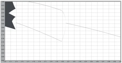
Next, we show the effect of %!. We choose the following parameters :
#!!!', $!!!%, $!!%!&, $"!"!&, '!!!#&, &!!!$, and #"!!!#. Figure
represents the bifurcation diagram for %! and shows the emergence of two-period
cycles depending on the values of %!. The vertical axis shows the value of
%&"!"%&""# and the horizontal axis shows the value of %!"!"%!"!!%#.
(a)#"!!!# (b)#"!!!#"
Figure : The dynamics of"%for each value of#"
When"!is sufficiently small, a unique limit point exists. When"!increases,
two-period cycles and endogenous fluctuations are observed. In addition, Figures (a)
and(b)depict the dynamics of "#. Figure (a)corresponds to the case in which
"!!!!"#; this shows that the steady state is stable and that the equilibrium path
fluctuates. Figure (b)corresponds to the case in which "!!!!"$; this shows
that the steady state is unstable and that two-period cycles emerge.
.Conclusion
In this study, we developed a variety-expansion growth model that integrated
the applied and basic research sectors to examine growth cycles. We show that the
equilibrium path can exhibit two-period cycles through the interplay between applied
and basic research. In addition, we explore the effects of change in basic research
spending and applied research subsidy. The steady-state growth rate increases when
basic research spending or applied research subsidy increases. However, the effects
on the possibility of cyclical instability differ by these two policies. An increase in
basic research spending reduces the possibility of cyclical instability, while an increase in applied research subsidy raises the possibility of cyclical instability.
(a)"!!!!"# (b)"!!!!"$ Figure : The dynamics of"#for each value of"!
Acknowledgments
I thank the participants at the th Workshop in Macroeconomics for Young
Economists and the Autumn Annual Meeting of the Japanese Economic
Association in Sophia University for their useful comments. This work was
supported by the Research Fellowship for Young Scientists of the Japan Society for
the Promotion of Science(JSPS)(No. J )and the Special Research
Grant from Matsuyama University. Any errors are my responsibility.
Appendix
A.Proof of LemmaDifferentiating Φ'%(with respect to λ yields
Λ Φ+'%(# '%( )'"'!!%!(&*'!"$"#"%$("" (A. ) Where Λ'%(&'$!'!!#"( #!% %#'!!%(#"')!!'!!%!(&*)!"'!!$($"#"%$* "'$!$"#"'!!#"(% #"$!! '!!%(#)#!$!'!!$(%*!
We differentiate Λ'%(with respect to λ as follows :
Λ+'%(#'%# #'!!#($!'!!#"( '!!%(#"! "$'!!$()!!'!!%!(&*$"#"%!!#"$ ! " "'$!$"#"'!!#"(% #"$!! '!!%(#)'#!$'#"$!!(!$'!!$(%*!
The second term’s entity within curly brackets is negative if #%$and #"$$!.
$!
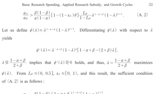
$"$&*"!&+%*"!%+,"!*"!'!+(- # "
"!#"'
"!%"&*"!'+%""! (A. )
Let us define )*'+''"!%"&*"!'+%"". Differentiating )*'+with respect to λ
yields
)/*'+$'!%"&*"!'+%,"!%"&!*#"&+'-!
λ㾶 "!%"&#"& implies that )/*'+㾷! holds, and thus, '$"!%"&
#"& maximizes
)*'+. From #")*!"!!$-, '!),!""+, and this result, the sufficient condition
of(A. )is as follows :
$!
$"$&*"!&+%*"!%+
"!%"& #"&
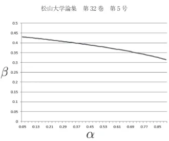
! ""!%"&!""%#"&"%""'Δ*%"&+! (A. )
Figure A. illustrates the combinations of α and β that maximize Δ*%"&+. By
using this result, we can depict the relation between α and the maximum value of
Δ*%"&+as shown in Figure A. . From Figure A. , Δ*%"&+is lower than one if
%),!!!$"!!%-. That is, the sufficient condition of(A. )is that !!!$%%%!!%
and $!&$". In summary, Λ/*'+#! holds if we assume that !##"%!!$,
!!!$%%%!!%,%&&, %"&%", and $!&$". Moreover, we investigate the value
of Λ*'+at '. !and '. "as follows :
'&(
'. !Λ*'+$"( $&% ''. "&(Λ*'+$!( (A. )
Hence, there is')which satisfies Λ *')+$!and '))*!""+. Because λ 㾶')implies
Λ*')+㾷 !, we obtain Φ/*'+㾷 ! when λ 㾶'). In addition, from (A. ) and
(A. ),'&(
'. !Φ
/*'+$"( holds, and thus, the steady-state '#$! is surely
We then consider the dynamic system when the applied research is not
conducted. From( ), differentiating Ψ$#%with respect to λ yields
Ψ&$#%#!"$!!"%#!"!#
"
$!"#!"!#"%" !
Figure A. : The combinations ofα and β that maximize Δ !!!""
Thus, !#Ψ*&''#"holds. By using( ), the properties of Φ &''and Ψ &''we
obtain
Φ&!'$! $&% Φ &"'$ )&"!('
&)"('&""$"#"'" (A. )
Ψ&!'$! $&% Ψ &"'$""$"
"#"! (A. )
(A. )and(A. )imply that Φ&"'#Ψ &"'holds. Therefore, we confirm that the
unique intersection of Φ&''and Ψ &''is in the region where !#'#".
B.Proof of Proposition
By using(A. )and( ), we obtain
Φ*&'#'$"!
&"!%'$!&"!#"' ' # "!'# ! "%
$!&"!#"'&'#'%&"!'#'"!%"("!&"!'!'()'#! &$
"#"&'#'& ""$"#"&'#'&!
Therefore, Φ*&'#'#"holds. If Φ*&'#'#!", the steady state is locally unstable.
On the other hand, if Φ*&'#'$!", the steady state is locally stable. From(A. )
and( ), we rearrange Φ*&'#'#!"as follows :
Γ&'#'%#)"&"!'!'(&"!)' "!#" " )$
!&%!'#'
&'#'"!%&"!'#'%"&"!&'()"&"!'
!'()$"#"&'#'& "!#" #!!
In contrast, Φ*&'#'$!"holds if Γ &'#'$!.
C.Derivation of the condition of( )
By using( ), the condition of('#"&()"&"!'
!'()%' # %'!$!is as follows : $!$&()"&"!'!'()&)""' &"!%')&"!#"' &' #'"!%&"!'#'% (C. )
Let us define&&''$'"!$&"!''$. Differentiating&&''with respect to λ yields
&*&''#'!$&"!''$!"&"!$!''!
λ㾶"!$ implies that &*&''㾷 ! holds, and thus, '#"!$ maximizes &&''.
From#"%&!"!!$), %!%(!""', and this result, the sufficient condition of(C. )
is as follows :
$!##%&)"('&)""'
&"!$') $$&"!$'"!$!
References
[ ] Aloi, M. and L. Lasselle( ) Growth and welfare effects of stabilizing innovation cycles. Journal of Macroeconomics , − .
[ ] Chu, A., G. Cozzi, and S. Galli( ) Does intellectual monopoly stimulate or stifle innovation ? European Economic Review , − .
[ ] Chu, A. and Y. Furukawa( ) Patentability and knowledge spillovers of basic R&D. Southern Economic Journal , − .
[ ] Cohen, W. M., R. R. Nelson, and J. P. Walsh( ) Links and impacts : the influence of public research on industrial R&D. Management Science , − .
[ ] Cozzi, G. and S. Galli( ) Science-based R&D in Schumpeterian growth. Scottish Journal of Political Economy , − .
[ ] Cozzi, G. and S. Galli( ) Privatization of knowledge : Did the U. S. get it right ? Economics Working Paper Series , University of St. Gallen, School of Economics and Political Science.
[ ] Cozzi, G. and S. Galli( ) Sequential R&D and blocking patents in the dynamics of growth. Journal of Economic Growth , − .
[ ] Deissenberg, C. and J. Nyssen( ) A simple model of Schumpeterian growth with complex dynamics. Journal of Economic Dynamics and Control , − .
[ ] Diamond, P. A.( ) National debt in a neoclassical growth model. American Economic
Review , − .
[ ] Francois, P. and H. Lloyd-Ellis( ) Animal spirits through creative destruction. American Economic Review , − .
[ ] Francois, P. and H. Lloyd-Ellis( ) Implementation cycles, investment, and growth. International Economic Review , − .
[ ] Francois, P. and H. Lloyd-Ellis( ) Schumpeterian cycles with pro-cyclical R&D. Review of Economic Dynamics , − .
[ ] Francois, P. and S. Shi( ) Innovation, growth, and welfare-improving cycles. Journal of Economic Theory , − .
[ ] Freeman, S., D. P. Hong, and D. Peled( ) Endogenous cycles and growth with indivisible technological developments. Review of Economic Dynamics , − .
[ ] Gale, D.( ) Delay and cycles. Review of Economic Studies , − .
[ ] Gersbach, H. and M. Schneider( ) On the global supply of basic research. Journal of Monetary Economics , − .
[ ] Gersbach, H., M. Schneider, and O. Schneller ( ) Basic research, openness, and convergence. Journal of Economic Growth , − .
[ ] Gersbach, H., G. Sorger, and C. Amon( ) Hierarchical growth : Basic and applied research. Journal of Economic Dynamics and Control , − .
[ ] Grandmont, J. M.( ) Nonlinear difference equations, bifurcations and chaos : An introduction. Research in Economics , − .
[ ] Griliches, Z.( ) Productivity, R&D, and basic research at the firm level in the s. American Economic Review , − .
[ ] Grossman, G. M. and E. Helpman( ) Innovation and growth in the global economy. MIT Press, Cambridge, MA.
[ ] Growiec, J. and I. Schumacher( ) Technological opportunity, long-run growth, and convergence. Oxford Economic Papers , − .
[ ] Haruyama, T.( ) R&D policy in a volatile economy. Journal of Economic Dynamics and Control , − .
[ ] Jaffe, A. B.( ) Real effects of academic research. American Economic Review , − .
[ ] Konishi, K.( ) Basic and applied research : A welfare analysis. Japanese Economic Review , − .
[ ] Li, B. and J. Zhang( ) Subsidies in an economy with endogenous cycles over investment and innovation regimes. Macroeconomic Dynamics , − .
[ ] Li, C. W.( ) Science, diminishing returns and long waves. Manchester School , − .
[ ] Mansfield, E.( ) Academic research and industrial innovation : An update of empirical findings. Research Policy , − .
[ ] Matsuyama, K.( ) Growing through cycles. Econometrica , − .
[ ] Park, W. G.( ) A theoretical model of government research and growth. Journal of Economic Behavior and Organization , − .
[ ] Shleifer, A.( ) Implementation cycles. Journal of Political Economy , − . [ ] Wälde, K.( ) Endogenous growth cycles. International Economic Review , −