I Introduction
In recent years, the development of the East Asian economy has attracted worldwide attention. Japan initially took the lead and achieved high economic growth in the 1960s. Japan was followed in the 1980s by the Asian Newly Industrializing Economies (NIEs), including South Korea, Singapore, Taiwan, and Hong Kong. In addition, China, India, and Vietnam have developed remarkably since the 1990s and have been supporters of the current high level of growth in the Asian economy.
However, the development of the East Asian economy has been far from smooth. The Asian financial crisis of 1997 had various impacts, not only on East Asian countries, but also on the world economy
Linkage of Stock Prices in Major Asian Markets
and the Asian and Global Financial Crises
*Abstract
The Asian financial crisis of 1997 and the global financial crisis have had various impacts on Asian countries through exchange rates, stock markets, and other elements. A consideration of the linkage between stock prices in Asian markets is indispensable if we are to plan ahead for the future of the Asian economy. In this paper, the linkage between stock prices for Asian markets such as Japan, Singapore, South Korea, the Chinese mainland, Hong Kong, and Taiwan since the 1990s is analyzed, as are the impacts of the Asian financial crisis and the global financial crisis on the Asian stock markets. The analysis demonstrates that the effects of the Japanese stock market and the Singapore stock market on the Asian markets are great, but the Chinese mainland market is little affected by other markets. On the whole, it has been revealed that the interdependence in stock prices among the Asian markets has increased since the global financial crisis.
Key Words: Linkage of Stock Prices, Asian Stock Markets, Asian Financial Crisis, Global Financial Crisis, Vector Autoregression (VAR) Model, Asian Economy
ZHANG, Yan
* The previous version of the paper was presented at the Asia-Pacific Economic Association Annual Conference, the Annual Meeting of Nippon Finance Association, and so on. I thank Kenjirou Hirayama (Kwansei Gakuin University), Toshino Serita (Aoyama Gakuin University), Toshiaki Watanabe (Hitotsubashi University), Young-Jae Kim (Pusan National University), Paul Vandenberg (Asian Development Bank), Lili Chen (Southwest University of Finance and Economics), and other participants for their helpful comments and suggestions. Of course, responsibility for any remaining errors is mine alone.
through exchange rates, stock markets, and other elements. In addition, the global financial crisis that arose from the subprime loan problem in the United States in 2007 hit East Asian economies through the global slowdown in demand.
The capital inflows and outflows of the East Asian stock markets continue in expectation of high Asian economic growth. The interdependence of stock markets is expected to increase as economic development and economic exchanges between the East Asian countries continue in the future. A consideration of the linkage between stock prices in East Asian markets is thus indispensable if we are to plan ahead for the future of the Asian economy. This analysis is also important for ascertaining the ideal way for the Asian economy to proceed.
There has been much previous research on the linkage of stock prices (for instance, Eun and Shin 1989, Chan et al. 1997, Ahlgren and Antell 2002, Forbes and Rigobon 2002, Wang et al. 2003, Boschi 2005, Fraser and Oyefeso 2005, and so on). Recent research on the linkage of stock prices in Asian markets includes the following: Chan et al. (1992) analyzed the relationships among the stock markets in Hong Kong, South Korea, Singapore, Taiwan, Japan, and the United States for 1983–1987. This paper used unit root tests and cointegration tests, and suggested that no evidence of cointegration was found. Hung and Cheung (1995) analyzed the interdependence of five major Asian emerging equity markets: Hong Kong, Korea, Malaysia, Singapore, and Taiwan, for 1981–1991. The paper used the Johansen multivariate cointegration approach, and suggested that the five Asian stock indices measured in local currency are not cointegrated, while the five Asian stock indices measured in terms of the US dollar are cointegrated. Corhay et al. (1995) analyzed the long run relationship among five major Pacific Basin stock markets, including Japan, Hong Kong, and Singapore, for 1972–1992. The paper used cointegration analysis, and found that there existed a rather integrated Pacific-Basin financial area. Sheng and Tu (2000) examined the linkages among the stock markets of 12 Asia–Pacific countries for the period from 1 July 1996 to 30 June 1998. This study used cointegration and variance decomposition analysis, and revealed the existence of cointegration relationships among these stock markets during the Asian financial crises. Yang et al. (2003) examined long-run cointegration relationships and short-run dynamic causal linkages among stock markets in the United States, Japan, and 10 Asian emerging stock markets, from 2 January 1995 to 15 May 2001. The paper employed a cointegrated vector autoregression (VAR) framework. The analyses showed that both long-run relationships and short-run linkages among these markets were strengthened during the Asian financial crisis, and that these markets have generally been more integrated after the crisis than before the crisis. Chen et al. (2007) analyzed the return and volatility interactions among Japan, Taiwan, South Korea and the US by employing a multivariate stochastic volatility (MSV) model. The data covered the period from January 1998 to December 2004. The analyses found no linkage of stock prices among these stock markets, although there was some linkage of stock prices between some markets. Huyghebaert and Wang (2010) examined the integration and causality of interdependencies among six major East Asian stock markets (Japan, Singapore, Hong Kong, Taiwan, South Korea, and
China) from 1 July 1992 to 30 June 2003. The study employed a Multivariate VAR model and showed that the integration of East Asian stock markets was strengthened during as well as after the Asian financial crisis. Cheng and Glascock (2005) analyzed the linkages among three Greater China Economic Area (GCEA) stock markets, including the Chinese mainland, Hong Kong, and Taiwan, and two developed markets, Japan and the US, over a period from January 1993 to August 2004. The study employed a GARCH model, an ARIMA model, and cointegration tests, and found that there was no evidence of cointegration among the GCEA, the Japan, and the U.S. markets.
The main contribution of this paper is that it is the first to analyze the linkage of stock prices in major East Asian markets, with the particular attention to both the 1997-1998 Asian financial crisis and the recent global financial crisis. Previous research on Asian stock markets has not analyzed the influence of the global financial crisis on the linkage of stock prices in major East Asian markets. The global financial crisis that occurred from the subprime loan problem of the United States had various impacts on not only the United States, but also Europe, Asia, and other areas, and caused the recent economic recession. Dooley and Hutchison (2009) analyzed transmission of the U.S. subprime crisis to emerging markets (Argentina, Brazil, Chile, Colombia, Mexico, China, South Korea, Malaysia, Czech Republic, Poland, Hungary, Russia, South Africa and Turkey) by focusing on 5-year Credit-default swap spreads on sovereign bonds. In this paper, the linkage between stock prices for East Asian markets such as Japan, Singapore, South Korea, the Chinese mainland, Hong Kong, and Taiwan since the 1990s is analyzed, as are the influences of both the Asian financial crisis and the global financial crisis on the East Asian stock markets.
The previous studies have analyzed long-run relationships and short-run dynamic causal linkages in the Asian stock markets. Some studies employed cointegration in order to investigate long-run relationships of the Asian stock markets (Chan et al. 1992, Corhay et al. 1995, Hung and Cheung 1995). Some studies have estimated short-run dynamic causal linkage (Sheng and Tu 2000). Some studies analyzed both long run relationships and short-run dynamic causal linkages, by employing vector autoregression (VAR) techniques, such as cointegration, impulse response analysis, and forecast error variance decomposition (Yang et al. 2003, Huyghebaert and Wang 2010), a GARCH model and an ARIMA model (Cheng and Glascock 2005), and a multivariate stochastic volatility model (MSV) (Chen et al. 2007). In this paper, in order to analyze the linkage of stock prices in major East Asian markets, vector autoregressive (VAR) techniques are used. According to Brooks (2008), VAR models have several advantages compared with univariate time series models or simultaneous equations structural models: (1) I do not need to specify which variables are endogenous or exogenous because all variables are endogenous; (2) VAR models allow the value of a variable to depend on more than just its own lags or combinations of white noise terms, so VAR models are more flexible than univariate AR models, and therefore can capture more features of the data; (3) The forecasts generated by VAR models are often better than ‘traditional structural’ models (Sims 1980).
The paper is organized as follows. First, the data are presented; a time series transition and the summary statistics are examined. Then, the methodology is introduced. Next, the empirical results of the unit root tests, cointegration tests, impulse response, and forecast error variance decomposition are reported. Finally, the summary and the concluding remarks are provided.
II Data
The data consist of day-end stock market index observations. This paper uses the Nikkei 225 Index (Japan), the Straits Times Index (Singapore), the Korea Composite Stock Price Index (South Korea), the Shanghai stock exchange composite index (Chinese mainland), the Hang Seng Index (Hong Kong), and the Taiwan Capitalization Weighted Stock Index (Taiwan) to analyze the linkage among stock prices in major East Asian markets. The indices are taken from the Nikkei NEEDS database and are corrected in logs. The sample period is from 1 January 1991 to 31 December 2010. The number of observations is 5219. The data are from Mondays to Fridays. If a value is missing, data of the previous day are used.
To examine the influence of the Asian financial crisis and the global financial crisis on the linkage of stock prices among the Asian markets, four periods are analyzed: before the Asian financial crisis, the period from 1 January 1991 to 30 June 1997; during the Asian financial crisis, the period from 1 July 1997 to 31 December 1998; after the Asian financial crisis and before the global financial crisis, the period from 1 January 1999 to 14 August 2007; 1 and after the global financial crisis, the period from 15 August 2007
to 31 December 2010.
2.1 A Time Series Transition of Stock Prices
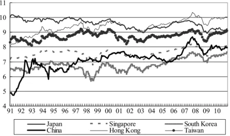
First, the movement of stock prices in each market is analyzed. Figure 1 shows a time series transition
4 5 6 7 8 9 10 11 91 92 93 94 95 96 97 98 99 00 01 02 03 04 05 06 07 08 09 10
Japan Singapore South Korea
China Hong Kong Taiwan
of stock prices in each market.
Figure 1 shows that, in general, stock prices in Japan have fallen. Although stock prices in Singapore and South Korea have risen gradually in the long term, stock prices fell sharply in 1998. Stock prices in Taiwan have risen gradually in the long term, although rises and falls occurred. Stock prices in China and Hong Kong have risen greatly over time, and stock prices in China have risen most rapidly of all. In addition, stock prices in all markets fell sharply from about October 2007 to February 2009.
2.2 Summary Statistics of Stock Prices
Table 1 displays the basic statistics describing stock prices. Table 1. Summary Statistics of Stock Prices
Table 1-1. Summary Statistics: sample: 1 January 1991 to 31 December 2010
Mean Std. Dev. Maximum Minimum
Japan 9.5966 0.3005 10.2090 8.8615 Singapore 7.5957 0.2768 8.2625 6.6909 South Korea 6.7722 0.4101 7.6328 5.6348 China 7.1461 0.7324 8.7147 4.6613 Hong Kong 9.3745 0.4579 10.3621 8.0010 Taiwan 8.7242 0.2478 9.2304 8.0506
Table 1-2. Summary Statistics: sample: 1 January 1991 to 30 June 1997
Mean Std. Dev. Maximum Minimum
Japan 9.8907 0.1279 10.2090 9.5687 Singapore 7.5385 0.2014 7.8215 7.0467 South Korea 6.6381 0.1909 7.0377 6.1292 China 6.3750 0.6580 7.3375 4.6613 Hong Kong 8.9373 0.4077 9.6288 8.0010 Taiwan 8.5708 0.2243 9.1083 8.0506
Table 1-3. Summary Statistics: sample: 1 July 1997 to 31 December 1998
Mean Std. Dev. Maximum Minimum
Japan 9.6850 0.1064 9.9318 9.4634 Singapore 7.2457 0.2441 7.6045 6.6909 South Korea 6.1195 0.2937 6.6615 5.6348 China 7.1115 0.0620 7.2584 6.9489 Hong Kong 9.2552 0.2250 9.7216 8.8039 Taiwan 8.9889 0.1168 9.2220 8.7406
Table 1-4. Summary Statistics: sample: 1 January 1999 to 14 August 2007
Mean Std. Dev. Maximum Minimum Rate of Change*
Japan 9.4782 0.2473 9.9443 8.9369 −4.2 Singapore 7.5832 0.2418 8.2066 7.1015 0.6 South Korea 6.7519 0.3262 7.6030 6.1501 1.7 China 7.3938 0.2854 8.4914 6.9192 16.0 Hong Kong 9.5080 0.2254 10.0636 9.0371 6.4 Taiwan 8.7328 0.2124 9.2304 8.1450 1.9
Note: This rate of change represents the rate of change compared with the mean from 1 January 1991 to 30 June 1997 (before the Asian financial crisis).
Table 1-5. Summary Statistics: sample: 15 August 2007 to 31 December 2010
Mean Std. Dev. Maximum Minimum Rate of Change*
Japan 9.2944 0.2123 9.7676 8.8615 −1.9 Singapore 7.8932 0.2241 8.2625 7.2841 4.1 South Korea 7.3718 0.1729 7.6328 6.8445 9.2 China 8.0110 0.2908 8.7147 7.4423 8.3 Hong Kong 9.9272 0.2110 10.3621 9.3071 4.4 Taiwan 8.8791 0.2124 9.1911 8.3163 1.7
Note: This rate of change represents the rate of change compared with the mean from 1 January 1999 to 14 August 2007 (after the Asian financial crisis and before the global financial crisis).
The rate of change of average stock prices from 1 January 1999 to 14 August 2007, was significantly higher compared with those from 1 January 1991 to 30 June 1997: with a difference of 16.0% in China and 6.4% in Hong Kong. The rate of change of average stock prices rose slightly: with a slight rise of 0.6% in Singapore, 1.7% in South Korea, and 1.9% in Taiwan. The rate of change of the average stock price in Japan fell by 4.2%.
In addition, the rate of change of average stock prices from 15 August 2007 to 31 December 2010, was higher compared with those from 1 January 1999 to 14 August 2007, although to different degrees: a difference of 4.1% in Singapore, 9.2% in South Korea, 8.3% in China, 4.4% in Hong Kong, and 1.7% in Taiwan. The rate of change of the average stock price in Japan fell by 1.9%.
III Methodology
In this section I describe the methodology utilized to conduct the empirical analyses of this paper. I start with describing the augmented Dickey-Fuller (ADF) and Phillips-Perron (PP) tests for unit roots. Next, I introduce Johansen test for cointegration. Further, I describe the impulse response functions and forecast error variance decomposition, two applications of the VAR model.
3.1 Unit Root Tests
To test whether the data series used is stationary, unit root tests are conducted. Here the unit root tests are carried out using the augmented Dickey-Fuller (ADF) and Phillips-Perron (PP) tests. 2
The two forms of the ADF test by Dickey and Fuller (1979, 1981) are given by the following equations:
(1) (2) where a0 is the drift term and a2 is the time trend. γ is the coefficient of the lagged dependent variable Xt−1. The ADF tests for stationarity are the ‘t’ tests on the coefficient γ. The critical values for the ADF tests are given in MacKinnon (1991). The null hypothesis is H0 : γ = 0. If this is true, Xt has a unit root. The lag length on these extra terms is either determined by the Akaike Information Criterion (AIC) or Schwartz Bayesian Criterion (SBC).
Phillips and Perron (1988) developed a generalization of the ADF test procedure that allows for fairly mild assumptions concerning the distribution of errors. The test regression for the Phillips-Perron (PP) test is as follows: (3) t i t P i i t t X X u X = + + ∆ + ∆ − = − 1 1 0 t i t P i i t t a X at X u X = + + + ∆ + ∆ − = − 1 2 1 0 t t t a X X = + + ∆ −1 0 −1
The PP statistics are just modifications of the ADF t statistics that take into account the less restrictive nature of the error process. The asymptotic distribution of the PP t statistic is the same as the ADF t statistic, therefore the critical values for the PP test is also given in MacKinnon (1991).
3.2 Cointegration Tests
To examine the long-term equilibrium relationships among the variables, cointegration tests are performed. Johansen (1988) derived the maximum likelihood estimator, which can estimate and test for the presence of multiple cointegrating vectors. 3
Following Johansen (1988) procedure, the augmented vector autoregressive (VAR) model can be written as follows:
(4) This can be rewritten as
(5) Where k g i a −i I =( =1 ) and g i j j i=( =1a −) I
The Johansen (1988) test focuses on an examination of the Π matrix. In equilibrium, all the ΔXt − i will be zero, and setting the error terms, εt , to their expected value of zero will leave ΠXt − k= 0, so Π can be interpreted as a long-run coefficient matrix.
There are two test statistics for cointegration under the Johansen approach, which are written as
and
Where r is the number of cointegrating vectors under the null hypothesis and i is the estimated value for the ith ordered eigenvalue from the Π matrix.
3.3 Generalized Impulse Response Functions
To analyze the influence among variables according to the VAR model, the impulse response is analyzed. An impulse response function traces the effect of a one-time shock to one of the innovations on current and future values of the endogenous variables. As with the impulse responses, the variance decomposition based on the Cholesky factor can change dramatically if the ordering of the variables is altered in the VAR, so the generalized impulse responses, not depending on the variable turns, are analyzed. Generalized Impulses as described in Pesaran and Shin (1998) constructs an orthogonal set of innovations
t k t k t t t aX aX a X X = 1 −1+ 2 −2+...+ − + t k t k t t k t t X X X X X = − + 1 −1+ 2 −2+...+ −1 −(−1)+ + = − − = g r i i trace r T In 1 ) ˆ 1 ( ) ( ) ˆ 1 ( ) 1 , ( 1 max r r+ =−TIn − r+
that is unaffected by ordering of variables. The VAR model is constructed as follows:
(6) where xt= (x1t, x2t,..., xmt)′ is an m×1 vector of jointly determined dependent variables, wt is an q×1 vector of deterministic and/or exogenous variables, and
{
i, =i ,12,...,p}
and ψ are m×m and m×q coefficient matrices.Under the assumption that all the roots of 0
1 = − = p i i i m z
I fall outside the unit circle, xt would be covariance-stationary, and (6) can be rewritten as the infinite moving average representation,
(7) where the m×m coefficient matrices Ai can be obtained using the following recursive relations:
(8) with A0=Im and Ai= 0 for i < 0, and Gi=Aiψ.
An impulse response function measures the time profile of the effect of shocks at a given point in time on the (expected) future values of variables in a dynamical system. The best way to describe an impulse response is to view it as the outcome of a conceptual experiment in which the time profile of the effect of a hypothetical m×1 vector of shocks of size =( 1,..., m)′, say, hitting the economy at time t is compared with a base-line profile at time t + n, given the economy’s history.
Denoting the known history of the economy up to time t – 1 by the non-decreasing information set Ωt–1, Pesaran and Shin (1998) proposed the generalized impulse response function (GI) of xt at horizon n as follows:
(9) Using (9) in (7), we have GIx(n, , t−1)=An , which is independent of Ωt–1, but depends on the composition of shocks defined by δ.
The Cholesky decomposition of Σ is as follows:
(10) where P is an m×m lower triangular matrix. Then, (7) can be rewritten as
(11) such that t=P−1 t are orthogonalized; namely,
m t
t I
E( ′)= . Hence, the m×1 vector of the orthogonalized impulse response function of a unit shock to the j th equation on xt+n is given by
, 1 t i t t p i i t x w x = − + + = , ,..., 2 , 1 T t = , 0 0 t i i i t i i i t A Gw x − ∞ = − ∞ = + = t =1,2,...,T, ( )=0, ( ′)= t t t E E , ... 2 2 1 1 i i p i p i A A A A = − + − + + − i= ,12,..., ) ( ) , ( ) , , ( t−1 = t+n t= t−1 − t+n t−1 x n E x E x GI , = ′ P P , ) ( ) ( ) ( 0 0 0 1 0 t i i i t i i i t i i i t i i i t AP P Gw AP Gw x − ∞ = − ∞ = − ∞ = − − ∞ = + = + = t =1,2,...,T,
(12) where ej is an m×1 selection vector with unity as its j th element and zeros elsewhere.
GI is defined as follows:
(13) Assuming that εt has a multivariate normal distribution, it is now easily seen that
(14) Hence, the m×1 vector of the (unscaled) generalized impulse response of the effect of a shock in the j th equation at time t on xt+n is given by
(15) By setting j= jj, the scaled generalized impulse response function is given by
(16) which measures the effect of one standard error shock to the j th equation at time t on expected values of x at time t + n.
3.4 Variance Decomposition
Variance decomposition separates the variation in an endogenous variable into the component shocks to the VAR. Thus, variance decomposition provides information about the relative importance of each random innovation in affecting the variables in the VAR.
The above generalized impulses can be used in the derivation of the forecast error variance decompositions, defined as the proportion of the n-step ahead forecast error variance of variable i which is accounted for by the innovations in variable j in the VAR. Denoting the orthogonalized and the generalized forecast error variance decompositions by o(n)
ij and ijg(n), respectively, then for n = 0,1,2,..., forecast error decomposition is as follows:
Notice that m=1 (n)=1 j o ij , and =1 ( )≠1 m j g
ij n due to the non-zero covariance between the original (non-orthogonalized) shocks. 4 , 0( ) j n j n =APe n=0, ,12,..., ) ( ) , ( ) , , ( j t−1 = t+n jt= j t−1 − t+n t−1 x n E x E x GI j jj j j jj mj j j j jt t e E 1 1 2 1, ,..., ) ( ) ( = = ′ − = − ), )( ( jj j jj j n e A ,..., 2 ,1 , 0 = n , ) ( 12 j n jj g j n = A e − ,..., 2 ,1 , 0 = n , ) ( ) ( ) ( 0 ′ 0 2 ′ = = = n l i l l i n l i l j o ij e A A e Pe A e n , ) ( ) ( ) ( 0 ′ ′ 0 2 ′ 1 = = − = n l i l l i n l i l j ii g ij e A A e e A e n i, =j 1,...,m ′
IV Empirical Results 4.1 Unit Root Tests
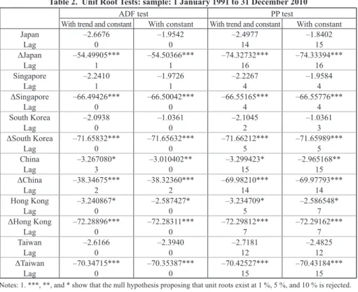
Here the unit root tests are carried out using the ADF tests and the PP tests for the two cases, with both a trend and a constant, and with a constant only. The unit root test results are presented in Table 2.
Table 2. Unit Root Tests: sample: 1 January 1991 to 31 December 2010
ADF test PP test
With trend and constant With constant With trend and constant With constant
Japan –2.6676 –1.9542 –2.4977 –1.8402 Lag 0 0 14 15 ΔJapan –54.49905*** –54.50366*** –74.32732*** –74.33394*** Lag 1 1 16 16 Singapore –2.2410 –1.9726 –2.2267 –1.9584 Lag 1 1 4 4 ΔSingapore –66.49426*** –66.50042*** –66.55165*** –66.55776*** Lag 0 0 4 4 South Korea –2.0938 –1.0361 –2.1045 –1.0361 Lag 0 0 2 3 ΔSouth Korea –71.65832*** –71.65632*** –71.66212*** –71.65989*** Lag 0 0 5 5 China –3.267080* –3.010402** –3.299423* –2.965168** Lag 3 0 15 15 ΔChina –38.34675*** –38.32360*** –69.98210*** –69.97793*** Lag 2 2 14 14 Hong Kong –3.240867* –2.587427* –3.234709* –2.586548* Lag 0 0 5 7 ΔHong Kong –72.28896*** –72.28311*** –72.29812*** –72.29162*** Lag 0 0 7 7 Taiwan –2.6166 –2.3940 –2.7181 –2.4825 Lag 0 0 12 12 ΔTaiwan –70.34715*** –70.35387*** –70.42527*** –70.43184*** Lag 0 0 15 15
Notes: 1. ***, **, and * show that the null hypothesis proposing that unit roots exist at 1 %, 5 %, and 10 % is rejected. 2. The lags are based on the Schwarz info criterion in the ADF tests and on the Newey–West bandwidth in the PP
tests.
The results indicate that the null hypotheses, namely, that unit roots are present, are rejected at the 10% significance level for the China and Hong Kong variables. The null hypotheses are not rejected at the 10% significance level for any of the other variables in any case. Moreover, the null hypotheses proposing that unit roots are present are all rejected at the 1% significance level in the first differences of the variables represented by Δ. That is, the first differences of the variables are all stationary, and all the variables are considered as I (1) processes. In the following analyses, the first differences are used to establish the stationarity of the data. 5
4.2 Cointegration Tests
Next, to establish whether cointegration exists between the stock prices, the Johansen test is employed. Table 3 presents the results.
Table 3. Cointegration Tests (Johansen’s likelihood ratio tests)
Table 3-1. Cointegration Tests: sample: 1 January 1991 to 31 December 2010 Null hypothesis Alternative hypothesis Trace test Max-eigenvalue test
r=0 r>=1 113.1(95.8) 54.0(40.1) r<=1 r>=2 59.1(69.8) 26.5(33.9) r<=2 r>=3 32.6(47.9) 13.7(27.6) r<=3 r>=4 19.0(29.8) 9.8(21.1) r<=4 r>=5 9.2(15.5) 7.6(14.3) r<=5 r>=6 1.6 (3.8) 1.6 (3.8)
Note: The figures in the parentheses represent 5% significance points.
Table 3-2. Cointegration Tests: sample: 1 January 1991 to 30 June 1997
Null hypothesis Alternative hypothesis Trace test Max-eigenvalue test
r=0 r>=1 68.1(95.8) 27.8(40.1) r<=1 r>=2 40.3(69.8) 15.1(33.9) r<=2 r>=3 25.3(47.9) 13.1(27.6) r<=3 r>=4 12.2(29.8) 7.6(21.1) r<=4 r>=5 4.6(15.5) 4.6(14.3) r<=5 r>=6 0.0 (3.8) 0.0 (3.8)
Table 3-3. Cointegration Tests: sample: 1 July 1997 to 31 December 1998
Null hypothesis Alternative hypothesis Trace test Max-eigenvalue test
r=0 r>=1 83.0(95.8) 28.8(40.1) r<=1 r>=2 54.2(69.8) 25.8(33.9) r<=2 r>=3 28.4(47.9) 13.5(27.6) r<=3 r>=4 14.9(29.8) 10.4(21.1) r<=4 r>=5 4.5(15.5) 4.1(14.3) r<=5 r>=6 0.4 (3.8) 0.4 (3.8)
Table 3-4. Cointegration Tests: sample: 1 January 1999 to 14 August 2007
Null hypothesis Alternative hypothesis Trace test Max-eigenvalue test
r=0 r>=1 91.8(95.8) 39.2(40.1) r<=1 r>=2 52.5(69.8) 22.8(33.9) r<=2 r>=3 29.7(47.9) 11.9(27.6) r<=3 r>=4 17.8(29.8) 10.2(21.1) r<=4 r>=5 7.6(15.5) 7.2(14.3) r<=5 r>=6 0.4 (3.8) 0.4 (3.8)
Table 3-5. Cointegration Tests: sample: 15 August 2007 to 31 December 2010 Null hypothesis Alternative hypothesis Trace test Max-eigenvalue test
r=0 r>=1 129.2(95.8) 42.4(40.1) r<=1 r>=2 86.8(69.8) 34.8(33.9) r<=2 r>=3 52.0(47.9) 28.3(27.6) r<=3 r>=4 23.7(29.8) 19.3(21.1) r<=4 r>=5 4.4(15.5) 4.0(14.3) r<=5 r>=6 0.3 (3.8) 0.3 (3.8)
Table 3-1 shows that both trace tests and max-eigenvalue tests found one cointegrating vector. Table 3-5 shows that trace tests found three cointegrating vectors. Table 3-2, Table 3-3, and Table 3-4 show that both trace tests and max-eigenvalue tests found no cointegrating vectors. In other words, generally speaking, for the period before the Asian financial crisis, the period of the Asian financial crisis, and the period after the Asian financial crisis and before the global financial crisis, no cointegration relationship existed among the markets. For the whole sample period and for the period after the global financial crisis,
cointegration relationships existed among the markets, and long-term equilibrium relationships could be found among the stock prices of these markets.
4.3 Impulse Response
First, I consider the trading time of each market before implementing the impulse response analysis. Figure 2 shows the stock trading opening and closing times in Japan standard time. The Tokyo market in Japan and the South Korea market open at 9 a.m., the Singapore market and the Taiwan market open at 10 a.m., the Shanghai market in China opens at 10:30 a.m., and the Hong Kong market opens at 11 a.m. In addition, the Taiwan market closes at 2:30 p.m., the Tokyo market and the South Korea market close at 3 p.m., the Shanghai market closes at 4 p.m., the Hong Kong market closes at 5 p.m., and the Singapore market closes at 6 p.m.
Figure 2. Stock trading opening and closing times (Japan standard time)
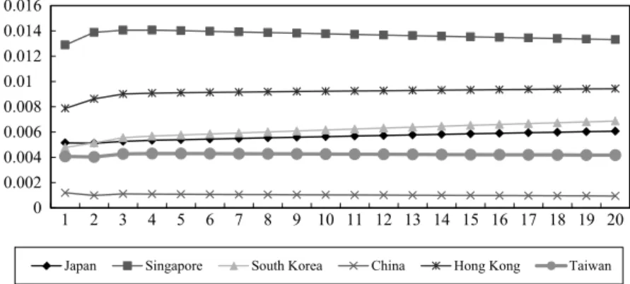
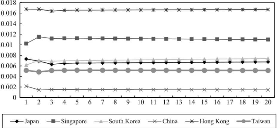
Here, the generalized impulse response, not depending on the variable turns, indicates the mechanism by which innovations in one stock market are transmitted to other markets over time. Figures 3-1 to 3-6 show the impulse responses of each market to a shock of one standard deviation. The vertical axes represent deviations from the trend, shown in percentage scale. The horizontal axes represent time, shown daily. Twenty days are represented. 6
Figure 3. Impulse Responses
Figure 3-1. Impulse Response of Japan: sample: 1 January 1991 - 31 December 2010 0 1 2 3 4 5 6 7 8 9 10 11 12 13 14 15 16 17 18 19 20 21 22 23 24
Tokyo Market Singapore Market
Korean Market Shanghai Market
Hong Kong Market Taiwan Market
Singapore Market South Korea Market
0 0.002 0.004 0.006 0.008 0.01 0.012 0.014 0.016 1 2 3 4 5 6 7 8 9 10 11 12 13 14 15 16 17 18 19 20 Japan Singapore South Korea China Hong Kong Taiwan
Figure 3-1 indicates the impulse response for Japan. It is as follows, in order of size. To a one standard deviation shock in its own value, the impulse response of Japan is 0.0148 on the first day and 0.0144 on the second day, settling at 0.014 beginning on the third day. To a one standard deviation shock in Hong Kong, the impulse response of Japan is 0.0065 on the first day, and settles at about 0.0071 beginning on the second day. To a one standard deviation shock in Singapore, it is 0.0059 on the first day and settles at 0.0074 beginning on the second day, exceeding the impulse response to a one standard deviation shock in Hong Kong on the second day. To a one standard deviation shock in South Korea, it is 0.0052 on the first day and settles at about 0.0059 beginning on the second day. To a one standard deviation shock in Taiwan, it is 0.0042 on the first day, 0.0046 on the second day, 0.0041 on the third day, and settles at 0.0042 beginning on the fourth day again. To a one standard deviation shock in China, the impulse response of Japan is 0.0012 on the first day, 0.0008 on the second day, and settles at 0.0009 beginning on the third day.
Figure 3-2. Impulse Response of Singapore: sample: 1 January 1991 - 31 December 2010
Figure 3-2 indicates the impulse response for Singapore. It is as follows, in order of size. To a one standard deviation shock in its own value, the impulse response of Singapore is 0.013 on the first day, settling at 0.014 beginning on the second day. To a one standard deviation shock in Hong Kong, the impulse response of Singapore is 0.008 on the first day, and settles at 0.009 beginning on the second day. To a one standard deviation shock in Japan, it is 0.0051 on the first two days, 0.0053 on the third day, and then becomes larger little by little until settles at 0.0061 on the twentieth day. To a one standard deviation shock in South Korea, the impulse response of Singapore is 0.0048 on the first day, 0.0051 on the second day, exceeding the shock of Japan on the second day, and then becomes larger little by little until settles at 0.0069 on the twentieth day. To a one standard deviation shock in Taiwan, it is 0.0041 on the first day, 0.0040 on the second day, and settles at about 0.0043 beginning on the third day. To a one standard deviation shock in China, the impulse response of Singapore is 0.0012 on the first day and settles at about 0.0010 beginning on the second day.
0 0.002 0.004 0.006 0.008 0.01 0.012 0.014 0.016 1 2 3 4 5 6 7 8 9 10 11 12 13 14 15 16 17 18 19 20 Japan Singapore South Korea China Hong Kong Taiwan
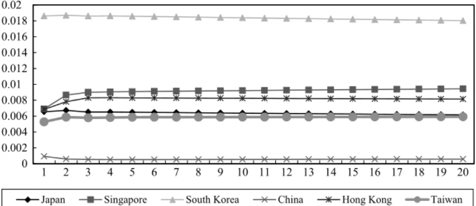
Figure 3-3. Impulse Response of South Korea: sample: 1 January 1991 - 31 December 2010
Figure 3-3 indicates the impulse response for South Korea. It is as follows, in order of size. To a one standard deviation shock in its own value, the impulse response of South Korea is 0.019 over time. To a one standard deviation shock in Singapore, it is 0.007 on the first day, and settles at 0.009 beginning on the second day. To a one standard deviation shock in Hong Kong, it is 0.007 on the first day, and settles at 0.008 beginning on the second day. To a one standard deviation shock in Japan, it is 0.0065 on the first day, 0.0067 on the second day, and then becomes smaller, settling at 0.0062 on the twentieth day. To a one standard deviation shock in Taiwan, the impulse response of South Korea is 0.005 on the first day, and settles at 0.006 beginning on the second day. To a one standard deviation shock in China, it is 0.0009 on the first day, and settles at about 0.0005 beginning on the second day.
Figure 3-4. Impulse Response of China: sample: 1 January 1991 - 31 December 2010
Figure 3-4 indicates the impulse response for China. It is as follows, in order of size. To a one standard deviation shock in its own value, the impulse response of China is 0.025 on the first day, and 0.026 on the second day, settling at 0.027 beginning on the third day. To one standard deviation shocks in other markets, the impulse responses of China are very small: concretely, to a one standard deviation shock in Hong Kong, the impulse response of China is about 0.0032, to a one standard deviation shock in
0 0.002 0.004 0.006 0.008 0.01 0.012 0.014 0.016 0.018 0.02 1 2 3 4 5 6 7 8 9 10 11 12 13 14 15 16 17 18 19 20
Japan Singapore South Korea China Hong Kong Taiwan
0 0.005 0.01 0.015 0.02 0.025 0.03 1 2 3 4 5 6 7 8 9 10 11 12 13 14 15 16 17 18 19 20
Singapore, it is about 0.0023, to a one standard deviation shock in Japan, it is also about 0.0020, to a one standard deviation shock in Taiwan, it is about 0.0016, and to a one standard deviation shock in South Korea, it is about 0.0012 over time.
Figure 3-5. Impulse Response of Hong Kong: sample: 1 January 1991 - 31 December 2010
Figure 3-5 indicates the impulse response for Hong Kong. It is as follows, in order of size. To a one standard deviation shock in its own value, the impulse response of Hong Kong is about 0.017 over time. To a one standard deviation shock in Singapore, the impulse response of Hong Kong is 0.010 on the first day, 0.012 on the second day, and settles at 0.011 beginning on the third day. To a one standard deviation shock in Japan, it is 0.0073 on the first day, 0.0070 on the second day, and settles at about 0.0063 beginning on the third day. To a one standard deviation shock in South Korea, it is 0.0062 on the first day, and settles at 0.0070 beginning on the second day, exceeding the impulse response of Hong Kong to a one standard deviation shock in Japan on the second day. To a one standard deviation shock in Taiwan, it is about 0.005 over time. To a one standard deviation shock in China, it is 0.002 on the first day and settles at 0.001 beginning on the second day.
Figure 3-6. Impulse Response of Taiwan: sample: 1 January 1991 - 31 December 2010 0 0.002 0.004 0.006 0.008 0.01 0.012 0.014 0.016 0.018 1 2 3 4 5 6 7 8 9 10 11 12 13 14 15 16 17 18 19 20
Japan Singapore South Korea China Hong Kong Taiwan
0 0.002 0.004 0.006 0.008 0.01 0.012 0.014 0.016 0.018 1 2 3 4 5 6 7 8 9 10 11 12 13 14 15 16 17 18 19 20
Figure 3-6 indicates the impulse response for Taiwan. It is as follows, in order of size. To a one standard deviation shock in its own value, the impulse response of Taiwan is 0.0160 on the first day and 0.0163 on the second day, settling at about 0.0168 beginning on the third day. To a one standard deviation shock in Singapore, it is 0.0051 on the first day, 0.0072 on the second day, and settles at about 0.008 beginning on the third day. To a one standard deviation shock in Hong Kong, it is 0.0049 on the first day, 0.0066 on the second day, and settles at 0.007 beginning on the third day. To a one standard deviation shock of South Korea, the impulse response of Taiwan is 0.0045 on the first day, and settles at 0.006 beginning on the second day. To a one standard deviation shock of Japan, the impulse response of Taiwan is 0.0045 on the first day, and settles at 0.006 beginning on the second day. To a one standard deviation shock in China, it is about 0.001 over time.
In summary, based on the impulse response, the effect of the Hong Kong market on the Singapore market is large, and at the same time, the effect of the Singapore market on the Hong Kong market is large. On the other hand, the Chinese market does not seem to have been much affected by the other stock markets. 4.4 Variance Decomposition
Forecast error variance decomposition is used to indicate the contribution of the innovation to the variation in each variable. The results are shown in Tables 4-1 to 4-6. In this case, 20 days are analyzed.
Table 4. Variance Decomposition (Unit: %)
Table 4-1. Variance Decomposition of Japan
1 January 1991 – 31 December 2010
Japan Singapore South Korea China Hong Kong Taiwan
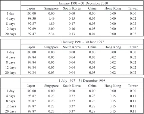
1 day 100.00 0.00 0.00 0.00 0.00 0.00 4 days 98.30 1.49 0.15 0.05 0.00 0.02 8 days 97.87 1.89 0.17 0.05 0.00 0.02 12 days 97.69 2.09 0.16 0.05 0.00 0.02 20 days 97.47 2.34 0.13 0.04 0.00 0.02 1 January 1991 – 30 June 1997
Japan Singapore South Korea China Hong Kong Taiwan
1 day 100.00 0.00 0.00 0.00 0.00 0.00 4 days 99.84 0.05 0.04 0.03 0.02 0.02 8 days 99.84 0.05 0.04 0.03 0.02 0.02 12 days 99.84 0.05 0.04 0.03 0.02 0.02 20 days 99.84 0.05 0.04 0.03 0.02 0.02 1 July 1997 – 31 December 1998
Japan Singapore South Korea China Hong Kong Taiwan
1 day 100.00 0.00 0.00 0.00 0.00 0.00
4 days 98.87 0.23 0.37 0.28 0.15 0.11
8 days 98.87 0.23 0.37 0.28 0.15 0.11
12 days 98.87 0.23 0.37 0.28 0.15 0.11
1 January 1999 – 14 August 2007
Japan Singapore South Korea China Hong Kong Taiwan
1 day 100.00 0.00 0.00 0.00 0.00 0.00 4 days 98.12 1.35 0.17 0.19 0.10 0.06 8 days 98.12 1.35 0.17 0.19 0.10 0.06 12 days 98.12 1.35 0.17 0.19 0.10 0.06 20 days 98.12 1.35 0.17 0.19 0.10 0.06 15 August 2007 – 31 December 2010
Japan Singapore South Korea China Hong Kong Taiwan
1 day 100.00 0.00 0.00 0.00 0.00 0.00
4 days 90.71 8.28 0.03 0.66 0.01 0.31
8 days 89.87 8.99 0.19 0.52 0.09 0.35
12 days 89.06 8.49 0.51 0.40 0.33 1.21
20 days 85.94 6.77 1.06 0.27 1.14 4.82
Table 4-1 shows the results of the variance decomposition for Japan from 1 January 1991 to 31 December 2010: for Japan, the variation of 100% depends on a shock from Japan itself on the first day, as does 97.5% on the 20th day. For the other five variables, the shocks of Singapore, South Korea, China, Hong Kong, and Taiwan on Japan account for only 2.34%, 0.13%, 0.04%, 0.00%, and 0.02%, respectively, on the 20th day, indicating that the degree to which these five markets influence Japan is very small.
Furthermore, after the global financial crisis, the period from 15 August 2007 to 31 December 2010, for Japan, its own shock decreased, but the shock of Singapore on Japan rose slightly. Therefore, it can be said that the Japan stock market has become easily affected by other markets because of the global financial crisis.
Table 4-2. Variance Decomposition of Singapore
1 January 1991 – 31 December 2010
Japan Singapore South Korea China Hong Kong Taiwan
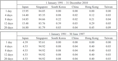
1 day 15.95 84.05 0.00 0.00 0.00 0.00 4 days 14.40 85.35 0.08 0.02 0.12 0.03 8 days 14.85 84.66 0.22 0.02 0.21 0.04 12 days 15.48 83.76 0.39 0.03 0.29 0.05 20 days 16.80 81.79 0.83 0.04 0.45 0.09 1 January 1991 – 30 June 1997
Japan Singapore South Korea China Hong Kong Taiwan
1 day 4.39 95.61 0.00 0.00 0.00 0.00
4 days 4.53 94.92 0.08 0.04 0.40 0.03
8 days 4.53 94.92 0.08 0.04 0.40 0.03
12 days 4.53 94.92 0.08 0.04 0.40 0.03
1 July 1997 – 31 December 1998
Japan Singapore South Korea China Hong Kong Taiwan
1 day 8.18 91.82 0.00 0.00 0.00 0.00 4 days 7.94 88.71 0.41 0.66 2.19 0.09 8 days 7.94 88.71 0.41 0.66 2.19 0.09 12 days 7.94 88.71 0.41 0.66 2.19 0.09 20 days 7.94 88.71 0.41 0.66 2.19 0.09 1 January 1999 – 14 August 2007
Japan Singapore South Korea China Hong Kong Taiwan
1 day 18.76 81.24 0.00 0.00 0.00 0.00 4 days 18.57 81.03 0.05 0.00 0.15 0.20 8 days 18.57 81.03 0.05 0.00 0.15 0.20 12 days 18.57 81.03 0.05 0.00 0.15 0.20 20 days 18.57 81.03 0.05 0.00 0.15 0.20 15 August 2007 – 31 December 2010
Japan Singapore South Korea China Hong Kong Taiwan
1 day 35.14 64.86 0.00 0.00 0.00 0.00
4 days 28.22 71.28 0.02 0.28 0.14 0.05
8 days 26.67 72.15 0.03 0.17 0.44 0.54
12 days 25.73 71.07 0.03 0.15 1.05 1.98
20 days 24.14 65.74 0.09 0.47 2.89 6.67
Table 4-2 shows the results of the variance decomposition for Singapore from 1 January 1991 to 31 December 2010: for Singapore, the variation of 81.79% depends on a shock from Singapore itself on the 20th day. Among the other five variables, the shock of Japan on Singapore accounts for 16.80% on the 20th day, indicating that the degree to which Japan influences Singapore is comparably large. The shocks of South Korea, China, Hong Kong, and Taiwan on Singapore account for only 0.83%, 0.04%, 0.45%, and 0.09%, respectively, on the 20th day; hence, it can be said that these four markets influence Singapore very little.
Furthermore, after the global financial crisis, for Singapore, its own shock decreased, but the shock of Japan on Singapore rose slightly. Therefore, it can be said that the Singapore stock market has become easily affected by other stock markets because of the global financial crisis.
Table 4-3. Variance Decomposition of South Korea
1 January 1991 – 31 December 2010
Japan Singapore South Korea China Hong Kong Taiwan
1 day 12.38 6.32 81.31 0.00 0.00 0.00
4 days 12.29 11.56 76.03 0.06 0.06 0.00
8 days 12.09 13.05 74.71 0.07 0.07 0.01
12 days 11.96 13.82 74.07 0.08 0.07 0.01
1 January 1991 – 30 June 1997
Japan Singapore South Korea China Hong Kong Taiwan
1 day 0.36 0.25 99.39 0.00 0.00 0.00 4 days 0.36 0.50 99.02 0.03 0.01 0.07 8 days 0.36 0.50 99.02 0.03 0.01 0.07 12 days 0.36 0.50 99.02 0.03 0.01 0.07 20 days 0.36 0.50 99.02 0.03 0.01 0.07 1 July 1997 – 31 December 1998
Japan Singapore South Korea China Hong Kong Taiwan
1 day 3.00 1.75 95.25 0.00 0.00 0.00 4 days 3.60 1.87 93.29 0.02 0.48 0.74 8 days 3.60 1.87 93.29 0.02 0.48 0.74 12 days 3.60 1.87 93.29 0.02 0.48 0.74 20 days 3.60 1.87 93.29 0.02 0.48 0.74 1 January 1999 – 14 August 2007
Japan Singapore South Korea China Hong Kong Taiwan
1 day 20.45 10.09 69.46 0.00 0.00 0.00 4 days 20.19 11.03 68.67 0.08 0.03 0.01 8 days 20.19 11.03 68.67 0.08 0.03 0.01 12 days 20.19 11.03 68.67 0.08 0.03 0.01 20 days 20.19 11.03 68.67 0.08 0.03 0.01 15 August 2007 – 31 December 2010
Japan Singapore South Korea China Hong Kong Taiwan
1 day 46.48 10.29 43.23 0.00 0.00 0.00
4 days 39.16 24.59 35.72 0.28 0.08 0.18
8 days 37.67 27.72 33.99 0.17 0.22 0.23
12 days 36.68 28.56 32.96 0.13 0.78 0.89
20 days 34.18 27.54 31.54 0.24 2.86 3.64
Table 4-3 shows the results of the variance decomposition for South Korea from 1 January 1991 to 31 December 2010: for South Korea, the variation of 81.31% depends on a shock from South Korea itself on the first day, as does 73.19% on the 20th day. Next to its own shock, the shocks of Singapore and Japan have comparably large effects on South Korea, accounting for 14.91% and 11.75%, respectively, on the 20th day. Hence, it can be said that the Singapore market and the Japan market influence the South Korea market. The shocks of China, Hong Kong, and Taiwan on South Korea account for only 0.08%, 0.06%, and 0.01%, respectively, on the 20th day, indicating that the degree to which these three markets influence South Korea is very small.
Furthermore, after the global financial crisis, for South Korea, its own shock decreased, but the shocks of Japan and Singapore on South Korea rose rapidly. Therefore, it can be said that the South Korea stock market has become easily affected by other stock markets because of the global financial crisis.
Table 4-4. Variance Decomposition of China
1 January 1991 – 31 December 2010
Japan Singapore South Korea China Hong Kong Taiwan
1 day 0.63 0.45 0.00 98.92 0.00 0.00 4 days 0.78 0.52 0.00 98.69 0.00 0.00 8 days 0.83 0.45 0.00 98.71 0.00 0.00 12 days 0.87 0.41 0.01 98.71 0.00 0.00 20 days 0.95 0.33 0.02 98.69 0.00 0.00 1 January 1991 – 30 June 1997
Japan Singapore South Korea China Hong Kong Taiwan
1 day 0.01 0.11 0.05 99.83 0.00 0.00 4 days 0.09 0.15 0.10 99.65 0.01 0.01 8 days 0.09 0.15 0.10 99.65 0.01 0.01 12 days 0.09 0.15 0.10 99.65 0.01 0.01 20 days 0.09 0.15 0.10 99.65 0.01 0.01 1 July 1997 – 31 December 1998
Japan Singapore South Korea China Hong Kong Taiwan
1 day 0.03 0.02 0.00 99.95 0.00 0.00 4 days 0.30 0.23 0.09 99.24 0.12 0.02 8 days 0.30 0.23 0.09 99.24 0.12 0.02 12 days 0.30 0.23 0.09 99.24 0.12 0.02 20 days 0.30 0.23 0.09 99.24 0.12 0.02 1 January 1999 – 14 August 2007
Japan Singapore South Korea China Hong Kong Taiwan
1 day 0.41 0.31 0.07 99.21 0.00 0.00 4 days 0.53 0.49 0.08 98.73 0.01 0.17 8 days 0.53 0.49 0.08 98.73 0.01 0.17 12 days 0.53 0.49 0.08 98.73 0.01 0.17 20 days 0.53 0.49 0.08 98.73 0.01 0.17 15 August 2007 – 31 December 2010
Japan Singapore South Korea China Hong Kong Taiwan
1 day 8.72 4.40 1.66 85.23 0.00 0.00
4 days 6.70 8.44 1.67 82.86 0.03 0.30
8 days 5.80 8.29 1.73 83.61 0.20 0.38
12 days 5.19 7.76 1.82 84.33 0.48 0.41
20 days 4.36 6.69 2.14 85.11 1.21 0.49
Table 4-4 shows the results of the variance decomposition for China from 1 January 1991 to 31 December 2010: for China, the variation of 98.92% depends on a shock from China itself on the first day, as does 98.69% on the 20th day. For the other five variables, the shocks of Japan, Singapore, South Korea, Hong Kong, and Taiwan on China account for only 0.95%, 0.33%, 0.02%, 0.00%, and 0.00%, respectively, on the 20th day, indicating that the degree to which these five markets influence China is very small.
Table 4-5. Variance Decomposition of Hong Kong
1 January 1991 – 31 December 2010
Japan Singapore South Korea China Hong Kong Taiwan
1 day 19.07 22.67 1.10 0.38 56.78 0.00 4 days 16.36 29.80 1.99 0.13 51.69 0.03 8 days 15.86 30.65 2.25 0.09 51.13 0.02 12 days 15.78 30.66 2.42 0.07 51.05 0.02 20 days 15.87 30.23 2.69 0.06 51.14 0.02 1 January 1991 – 30 June 1997
Japan Singapore South Korea China Hong Kong Taiwan
1 day 3.77 15.44 0.07 0.00 80.72 0.00 4 days 3.76 15.70 0.11 0.00 80.37 0.06 8 days 3.76 15.70 0.11 0.00 80.37 0.06 12 days 3.76 15.70 0.11 0.00 80.37 0.06 20 days 3.76 15.70 0.11 0.00 80.37 0.06 1 July 1997 – 31 December 1998
Japan Singapore South Korea China Hong Kong Taiwan
1 day 14.85 26.37 0.35 0.29 58.14 0.00 4 days 14.61 25.50 1.79 2.02 55.81 0.28 8 days 14.61 25.50 1.79 2.02 55.81 0.28 12 days 14.61 25.50 1.79 2.02 55.81 0.28 20 days 14.61 25.50 1.79 2.02 55.81 0.28 1 January 1999 – 14 August 2007
Japan Singapore South Korea China Hong Kong Taiwan
1 day 22.75 18.69 3.64 0.39 54.52 0.00 4 days 22.59 19.33 3.66 0.56 53.62 0.25 8 days 22.59 19.33 3.66 0.56 53.62 0.25 12 days 22.59 19.33 3.66 0.56 53.62 0.25 20 days 22.59 19.33 3.66 0.56 53.62 0.25 15 August 2007 – 31 December 2010
Japan Singapore South Korea China Hong Kong Taiwan
1 day 39.17 25.03 1.45 4.99 29.37 0.00
4 days 33.05 44.60 1.29 1.76 19.02 0.29
8 days 31.38 49.66 0.92 1.69 16.04 0.32
12 days 30.28 51.93 0.70 2.21 13.85 1.03
20 days 28.26 52.59 0.51 4.11 10.60 3.93
Table 4-5 shows the results of the variance decomposition for Hong Kong from 1 January 1991 to 31 December 2010: for Hong Kong, the variation of 56.78% depends on a shock from Hong Kong itself on the first day, as does 51.14% on the 20th day. Next to its own shock, the shocks of Singapore and Japan on Hong Kong account for 30.23% and 15.87%, respectively, on the 20th day; hence, it can be said that the Singapore market and the Japan market influence the Hong Kong market. The shocks of South Korea, China, and Taiwan on Hong Kong account for only 2.69%, 0.06%, and 0.02%, respectively, on the 20th day, indicating that the degree to which these three markets influence the Hong Kong market is very small.
of Singapore and Japan rose. Therefore, it can be said that the Hong Kong stock market has become easily affected by other stock markets because of the global financial crisis.
Table 4-6. Variance Decomposition of Taiwan
1 January 1991 – 31 December 2010
Japan Singapore South Korea China Hong Kong Taiwan
1 day 7.96 4.94 2.03 0.07 0.68 84.33 4 days 11.20 9.95 2.20 0.02 1.10 75.52 8 days 11.77 11.00 2.26 0.01 1.22 73.74 12 days 11.99 11.29 2.31 0.01 1.27 73.14 20 days 12.22 11.44 2.39 0.01 1.32 72.62 1 January 1991 – 30 June 1997
Japan Singapore South Korea China Hong Kong Taiwan
1 day 0.86 1.31 0.03 0.00 0.44 97.35 4 days 1.27 1.91 0.05 0.00 0.46 96.30 8 days 1.27 1.91 0.05 0.00 0.46 96.30 12 days 1.27 1.91 0.05 0.00 0.46 96.30 20 days 1.27 1.91 0.05 0.00 0.46 96.30 1 July 1997 – 31 December 1998
Japan Singapore South Korea China Hong Kong Taiwan
1 day 2.68 7.45 0.17 0.07 1.73 87.90 4 days 4.13 8.64 0.87 0.42 2.24 83.70 8 days 4.13 8.64 0.87 0.42 2.24 83.70 12 days 4.13 8.64 0.87 0.42 2.24 83.70 20 days 4.13 8.64 0.87 0.42 2.24 83.70 1 January 1999 – 14 August 2007
Japan Singapore South Korea China Hong Kong Taiwan
1 day 9.36 4.54 4.49 0.05 0.22 81.34 4 days 9.94 5.43 4.48 0.07 0.61 79.47 8 days 9.94 5.43 4.48 0.07 0.61 79.47 12 days 9.94 5.43 4.48 0.07 0.61 79.47 20 days 9.94 5.43 4.48 0.07 0.61 79.47 15 August 2007 – 31 December 2010
Japan Singapore South Korea China Hong Kong Taiwan
1 day 31.90 9.13 8.60 0.35 0.31 49.70
4 days 33.52 20.54 6.20 0.11 0.49 39.14
8 days 32.14 20.61 6.47 0.18 0.28 40.31
12 days 30.52 18.97 7.16 0.40 0.51 42.44
20 days 27.38 15.19 9.42 1.12 2.03 44.86
Table 4-6 shows the results of the variance decomposition for Taiwan from 1 January 1991 to 31 December 2010: for Taiwan, the variation of 84.33% depends on a shock from Taiwan itself on the first day, as does 72.62% on the 20th day. Next to its own shock, the shocks of Japan and Singapore on Taiwan account for 12.22% and 11.44%, respectively, on the 20th day; hence, it can be said that the Japan market and the Singapore market influence the Taiwan market. The shocks of South Korea, China and Hong
Kong on Taiwan account for only 2.39%, 0.01%, and 1.32%, respectively, on the 20th day, indicating that the degree to which these three markets influence Taiwan is very small.
Furthermore, after the global financial crisis, the period from 15 August 2007 to 31 December 2010, for Taiwan, its own shock decreased, but the shock of Japan rose. Therefore, it can be said that the Taiwan stock market has become easily affected by other stock markets because of the global financial crisis.
The results of the above-mentioned variance decomposition are as follows: the Singapore market and the Japan market considerably influenced the other Asian markets, including the markets of South Korea, Hong Kong, and Taiwan. Furthermore, the Asian stock markets have become easily affected by other stock markets because of the global financial crisis.
V Summary and Concluding Remarks
In this paper, the linkage of stock prices in East Asian markets (including Japan, Singapore, South Korea, China, Hong Kong, and Taiwan) since the 1990s was analyzed, as well as the influences of the Asian financial crisis and the global financial crisis on the East Asian stock markets.
In line with Sheng and Tu (2000), Yang et al. (2003), and Huyghebaert and Wang (2010), I did observe that the linkage of stock prices in the Asian markets had increased during the 1997-1998 Asian financial crisis by using correlation analysis, a straightforward measure. However, by using cointegration tests, impulse response, and forecast error variance decomposition, I could not find that the linkage had increased during the period of the Asian financial crisis clearly. Furthermore, according to all analyses results, my result demonstrated that the linkage of stock prices in the East Asian markets had increased since the global financial crisis.
Unlike Huyghebaert and Wang (2010), who points out that the Singapore and Hong Kong stock markets are two interactive and influential markets in the region during and after the Asian financial crisis, and unlike Dekker et al. (2001), who indicates that Hong Kong is the leading market, my finding indicates that the effects of the Japanese stock market and the Singapore stock market on the Asian markets are great. I cannot get the conclusion that Hong Kong turned out to be a very important financial center in the East Asian region.
In line with Huyghebaert and Wang (2010), my analysis further demonstrates that the Chinese mainland market is little affected by other markets. As for the Chinese mainland market, the reason the influence from other countries is small is thought to be that capital transactions are not currently liberalized in China. The majority of investors in the Chinese mainland stock market are domestic investors; foreigner investors cannot yet invest freely. In addition, the investment in overseas assets is limited to the Chinese mainland domestic investors. The Chinese mainland market is basically speculative; domestic investors do not pass the judge investments based on fundamentals like the corporate performance, but simply seek capital gains.
Slowdown of the real economy is currently of concern in the Asian region due to the global financial crisis. Due to the advancement of globalization, impacts in one country in the field of finance immediately spread to other countries. The Asian financial markets have now developed into an important part of the global market. However, it cannot yet be said that the arbitrage and adjustment functions of the Asian financial markets are sufficient. Because the degree of enterprises’ dependence on bank loans remains high, it is necessary to make efforts to develop the stock markets more in the Asian countries, to diversify the financing of enterprises and the choice of investments, and to use risk analysis to exchange information more widely in the future. To overcome the global financial crisis now, Asian countries should not only strengthen their economic fundamentals and implement structural reform, but also respond jointly to financial risk. If they do so, we can expect the financial liberalization and unification of the Asian economy to advance smoothly, and the financial system to be strengthened further.
Notes
1 BNP Paribas, a bank major company in France, froze the subsidiary fund due to the US subprime loan problem on 15 August 2007, so the subprime loan problem came up.
2 The unit root test approach refers to Asteriou and Hall (2007). 3 The Johansen test approach refers to Brooks (2008).
4 If the variables in a VAR model are cointegrated, then Vector Error Correction Model (VECM) should be used to estimate the impulse response and variance decomposition.
5 The first difference of the stock prices that took a natural logarithm becomes approximately the rate of stock returns.
6 According to the Akaike information criterion, the VAR order lag is two period lags. References
Ahlgren, N. and Antell, J., 2002. Testing for Cointegration between International Stock Prices. Applied Financial Economics, 12 (12), 851-861.
Asteriou, D. and Hall, S. G., 2007. Applied Econometrics: A Modern Approach Using EViews and Microfit Revised Edition. Palgrave Macmillan, 297-299.
Boschi, M., 2005. International Financial Contagion: Evidence from the Argentine Crisis of 2001-2002. Applied Financial Economics, 15 (4), 153-163.
Brooks, C., 2008. Introductory Econometrics for Finance. Cambridge University Press, 291-292.
Chan, K.C., Gup, B.E. and Pan, M.S., 1992. An Empirical Analysis of Stock Prices in Major Asian Markets and the United States. The Financial Review, 27 (2), 289-307.
Chan, K.C., Gup, B.E. and Pan, M.S., 1997. International Stock Market Efficiency and Integration: A Study of Eighteen Nations. Journal of Business Finance & Accounting, 24 (6), 803-813.
Chen, S.L., Huang, S.C. and Lin, Y.M., 2007. Using Multivariate Stochastic Volatility Models to Investigate the Interactions among NASDAQ and Major Asian Stock Indices. Applied Economics Letters, 14 (2), 127-133. Cheng, H. and Glascock, J.L., 2005. Dynamic Linkages between the Greater China Economic Area Stock Markets—
Mainland China, Hong Kong, and Taiwan. Review of Quantitative Finance and Accounting, 24, 343-357. Corhay, A., Rad, A.T. and Urbain, J.P., 1995. Long Run Behaviour of Pacific-Basin Stock Prices. Applied Financial
Economics, 5 (1), 11-18.
Dekker, A., Sen, K. and Young, M., 2001. Equity Market Linkages in the Asia Pacific Region: A Comparison of the Orthogonalized and Generalized VAR Approaches. Global Finance Journal, 12 (1), 1-33.
Dickey, D.A. and Fuller, W.A., 1979. Distribution of the Estimators or Autoregressive Time Series with a Unit Root. Journal of the American Statistical Association, 74 (366), 427-431.
Dickey, D.A. and Fuller, W.A., 1981. Likelihood Ratio Statistics for Autoregressive Time Series with a Unit Root. Econometrica, 49 (4), 1057-1072.
Dooley, M.P. and Hutchison, M.M., 2009. Transmission of the U.S. Subprime Crisis to Emerging Markets: Evidence on the Decoupling-Recoupling Hypothesis. NBER Working Paper 15120.
Eun, C.S. and Shin, S., 1989. International Transmission of Stock Market Movements. Journal of Financial and Quantitative Analysis, 24 (2), 241-256.
Forbes, K.J. and Rigobon, R., 2002. No Contagion, Only Interdependence: Measuring Stock Market Comovements. The Journal of Finance, 57 (5), 2223-2261.
Fraser, P. and Oyefeso, O., 2005. US, UK and European Stock Market Integration. Journal of Business Finance & Accounting, 32 (1&2), 161-181.
Hung, B.W. and Cheung, Y.L., 1995. Interdependence of Asian Emerging Equity Markets. Journal of Business Finance and Accounting, 22 (2), 281-288.
Huyghebaert, N. and Wang, L.H., 2010. The Co-movement of Stock Markets in East Asia: Did the 1997–1998 Asian Financial Crisis Really Strengthen Stock Market Integration? China Economic Review, 21, 98-112.
Johansen, S., 1988. Statistical Analysis of Cointegration Vectors. Journal of Economic Dynamics and Control, 12, 231-254.
MacKinnon, J.G., 1991. Critical Values for Cointegration Tests. In: Engle, R.F. and Granger, C.W.J., eds. Long-Run Economic Relationships: Readings in Cointegration, Oxford University Press, 267-276.
Pesaran, H.H. and Shin,Y., 1998. Generalized Impulse Response Analysis in Linear Multivariate Models. Economics Letters, 58 (1), 17-29.
Phillips, P.C.B. and Perron, P., 1988. Testing for a Unit Root in Time Series Regression. Biometrika, 75 (2), 335-346.
Sheng, H.C. and Tu, A.H., 2000. A Study of Cointegration and Variance Decomposition among National Equity Indices before and during the Period of the Asian Financial Crisis. Journal of Multinational Financial Management, 10, 345-365.
Sims, C.A., 1980. Macroeconomics and Reality. Econometrica, 48, 1-48.
Wang, Z., Yang, J. and Bessler, D.A., 2003. Financial Crisis and African Stock Market Integration. Applied Economics Letters, 10 (9), 527-533.
Yang, J., Kolari, J.W. and Min, I., 2003. Stock Market Integration and Financial Crises: The Case of Asia. Applied Financial Economics, 13 (7), 477-486.