機械学習に基づく決定性の中国語依存構造解析器

全文

(1)2004−ＦＩ− 76 (13) 2004−ＮＬ−163 (13) 2004／9／17. 社団法人情報処理学会研究報告 IPSJ SIG Technical Report. 機械学習に基づく決定性の中国語依存構造解析器鄭育昌浅原正幸松本裕治奈良先端科学技術大学院大学情報科学研究科 {yuchan-c, masayu-a, matsu}@is.naist.jp 概要：本研究では、機械学習に基づく決定性の中国語依存構造解析器を実装する。依存構造解析アルゴリズムとして山田モデルと Nivre モデルを用いて実装し、構造を判別する機械学習器として最大エントロピー法と SVM 法を用いた。本稿では、CKIP treebank を用いて各モデルの有効性について比較検証する。実験結果によると、Nivre モデルは山田モデルで残されている曖昧性を解決できる。その他、中国語に存在する多様な複合名詞問題に対して、chunker を用いた複合名詞抽出による精度向上についても検討する。. Machine Learning-based Dependency Analyzer for Chinese Yuchang CHENG, Masayuki ASAHARA, Yuji MATSUMOTO Graduate School of Information Science Nara Institute of Science and Technology {yuchan-c, masayu-a, matsu}@is.naist.jp Abstract: In this paper, we present a deterministic dependency structure analyzer for Chinese. This analyzer implements two algorithms – Yamada and Nivre model – and two sorts of classifier – SVMs and MaxEnt. We compare the performance of two algorithms (by Yamada and by Nivre). We evaluate the method on a dependency tagged corpus derived from the CKIP Treebank corpus. The result shows that Nivre’s algorithm can resolve some problems in Yamada’s algorithm. Then we try to add NP-chunker in our analyzer. Although the result of NP-chunker experiment doesn’t show significantly better performance, we discuss that using NP-chunker is necessary for Chinese dependency analyzing.. 1. Introduction. Many syntactic analyzers for English have been implemented and have demonstrated good performance (Charniak, 2000; Collins, 1997; Ratnaparkhi, 1999). However, implementation of Chinese syntactic structure analyzers is still limited, since the structure of the Chinese language is quite different from other languages. We are currently developing a Chinese syntactic structure analyzer. In this paper, we present our machine learning-based syntactic structure analyzer for Chinese. Our analyzer produces word dependency structure rather than phrase structures. The reason is that dependency structures are simpler and more comprehensible than phrase structures. Moreover, construction of a word dependency annotated. corpus is easier than construction of a phrase structure annotated corpus for use as the training data. Consistency among annotators can also be more easily achieved using the simpler dependency structure. We utilize a deterministic method for dependency relation construction. One approach is a generative dependency structure analysis consisting of two steps: First, a dependency relation matrix is constructed, in which each element corresponds to a pair of tokens. The dependency relation between each pair is assigned a likelihood value. Second, the optimal dependency structure is estimated using the likelihood of the whole sentence under no-crossing constraint. The other approach, a deterministic dependency structure analysis, is proposed for Japanese (Kudo, 2002) and for English (Yamada, 2003). We adopt. 1 −91−.

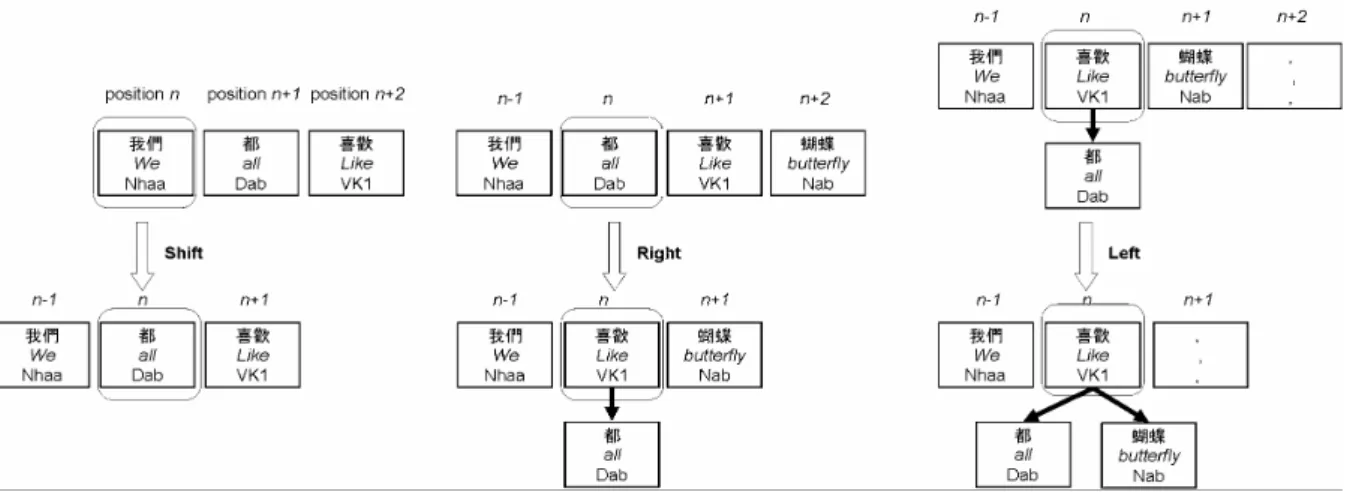
(2) Figure 1: Three operations of Yamada’s model. Yamada’s method to Chinese dependency analysis. However, Yamada’s method still has a crucial ambiguity to estimate the parsing actions. Machine learner cannot estimate the actions with the surrounding features. To resolve the problem, we implement another bottom-up algorithm proposed by (Nivre, 2004). Nivre’s method is applied to Norwegian and based on memory-based learning. In Yamada’s algorithm and Nivre’s algorithm, the dependency relations are composed by a bottom-up schema with machine learners. We incorporate Support Vector Machines (hereafter SVMs) and Maximum Entropy (hereafter MaxEnt) models into their algorithms. There are many nominal compounds in Chinese, which include more than three words in many cases. However, our analyzer cannot analyze these long nominal compounds well. Then, we adopt an NP-chunker based on SVMs to extract nominal compounds from the input sentence before dependency analysis. We compare the accuracy of two approaches. The aim is to implement a variation of the deterministic method and to show how the method is applicable to Chinese dependency analysis. Our analyzer is experimented on the CKIP Chinese Treebank (K-J Chen et al, 1999), which is a phrase structured and head annotated corpus. The phrase structure is converted into a dependency structure according to the head information. We perform experimental evaluations in several settings on the converted corpus. In the next section, we describe two deterministic dependency structure analysis algorithms. Section 3 reports experimental evaluation and comparison with related work. Section 4 discusses the errors in our experiments and the effect of NP-chunker in the reduction of errors.. Finally, we summarize our findings in the conclusion.. 2. Parsing Models. This section presents two parsing algorithms proposed by (Yamada, 2003) and (Nivre, 2004). Both algorithms are deterministic approaches, in which the dependency relations are constructed by a bottom-up deterministic schema. The algorithm uses two major procedures: (i) Extract the surrounding features for the focused node (or node pair). (ii) Estimate the dependency relation operation for the focused node by a machine learning method. First, we describe these algorithms. Second, we discuss the difference between two algorithms.. 2.1. Parsing Algorithm. 2.1.1 Yamada’s algorithm In Yamada’s algorithm (Yamada, 2003), a dependency relation for each word position is represented by the following three operations: Shift, Left and Right. The operation is determined by a classifier, SVMs, based on the surrounding features. The determination is iterated until the classifier cannot make any further dependency relation on the whole sentence. The details of the three operations are as follows: Shift means that there is no relation between the focused node and the preceding (left) or the succeeding (right) node. In this case, the focused node moves to the succeeding node. The left figure in Figure 1 illustrates the shift operation, which the focused node is shown in a round box. In this operation, no dependency relation is constructed. Right means that the focused node becomes a child of the succeeding node. The center figure in Figure 1 illustrates the right operation.. 2 −92−.

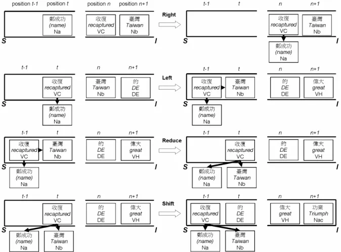
(3) Left means that the focused node becomes a child of the preceding node. The right figure in Figure 1 illustrates the left operation. Note that once either Left or Right operation is applied, the focused node becomes a child of another node and will never be considered in future analysis. In other words, the focused node cannot receive any nodes as its child. To check the child to be complete, the classifier utilizes surrounding features which are discussed in the section 3.1.2. 2.1.2 Nivre’s algorithm In Nivre’s algorithm (Nivre 2004), the analyzer configurations are represented by a triple S , I , A . S is a stack, I is a list of remaining input tokens, and A is a list of dependency relations. Given an input token sequences W, the analyzer is initialized the triple as nil ,W , φ . The analyzer will estimate the dependency relation between two tokens (the latest token t in S and the first token n. in I). The algorithm will iterate until the list I becomes empty. When the list I becomes empty, the analyzer stops the iteration and outputs the word dependency relation. There are four possible operations to the next configuration: Right: In the current triple t | S , n | I , A , if there is a dependency relation that the word t depends on word n , extend A with (t → n ) , remove t from S, and give the triple S , n | I , A U {(t → n )} Left: In the current triple t | S , n | I , A , if there is a dependency relation that the word n depends on the word t, extend A with (n → t ) , push n onto the stack S, and give the triple n | t | S , I , A U {(n → t )} . In the current triple t | S , n | I , A , if there is no dependency between n and t, check the conditions of the actions below; Reduce: If there are no more words n' ∈ I de-. Figure 2: Four operations of Nivre’s algorithm. Example: 鄭成功收復臺灣的偉大功業(“The great triumph that Cheng Kheng-Koug recaptured Taiwan.”). 3 −93−.

(4) pends on t, and t has a parent on its left side; analyzer removes t from the stack S, and give the triple S , n | I , A Shift: If there is no dependency between n and t, and the triple doesn’t satisfy the conditions in Reduce, then push n onto the stack S, and give the triple n | t | S , I , A . These operations are depicted in Figure 2. Given an input sentence of length N (words), the analyzer is guaranteed to terminate after at most 2N actions. The dependency structure given at the termination is well-formed if and only if the subtrees are connected (Nivre, 2004). This means that it is a set of connected components, each of which is a well-formed dependency graph for a subtree of the input sentence. It should be noted that the definition above is presented differently to the original algorithm (Nivre, 2004). Similar to Yamada’s algorithm, each word of input sentence becomes a token. The token includes the word, the POS, the information about its children, and other useful information. These becomes the features for the classifier. 2.1.3 Comparison between the two algorithms In the Yamada’s algorithm, the operation Shift means not only “The focused node doesn’t dependent on the preceding (left adjacent) or the succeeding (right adjacent) node” but also “It depends on the left adjacent, but the operation should be delayed since there is a possibility that some node on the right side may depend on the node. Therefore it should remain in token sequence”. If the focused node has a potential child on the right side and the child hasn’t been analyzed yet, the current node should wait for the child to be analyzed. However, if the focused node depends on the left node and it becomes a child of the preceding node, the latter nodes may be lost the correct dependencies. In (Cheng, 2004), we arranged for the training data to let classifier predict correct operation (Left or Shift). However, there is high ambiguity in Shift operation. The ambiguity of Shift is a crucial error source in their experiment. By contrast, there are four operations in Nivre’s algorithm. If the current triple has a dependency relation, it must be extended to A. Even the relation is (n → t ) , the word n will be pushed onto S. This approach guarantees that the succeeding words can depend on n and don’t lost the relation. (n → t ) . This algorithm can resolve some problems about the ambiguity of Shift operation (in Yamada’s algorithm). However, if the word n has no more children in the succeeding words, it should select Reduce operation after the word n be pushed onto S. If it doesn’t select Reduce operation, the succeeding words in I supposedly depend on wrong word. This is a major error source in our experiment discussing in Section 4. However, the result shows that the Nivre’s algorithm can get better performance.. 2.2. Machine Learning Models. In Yamada’s method (Yamada, 2003), the operation is determined by SVMs (Vapnik, 1998). Alternative, Nivre’s method uses memory-based learning to determine the operations. In our method, we use SVMs and MaxEnt method for machine learning in both algorithms. SVMs are a binary classifier based on a maximum margin strategy. In our preceding experiment (Cheng, 2004), we use the polynomial kernel: K ( x, z ) = (1 + x ⋅ z ) d . To extend binary classifiers to multi-class classifiers, we use a pair-wise method which utilizes n C 2 binary classifiers between all pairs of the classes (Kreel, 1998). In our experiment with Yamada’s algorithm, when the training data size is more than 90,000 words, the machine leaning can’t converge. Similarly, this problem exists in our experiment with Nivre’s algorithm. Therefore, we implement MaxEnt method in both algorithms. MaxEnt model is a statistical approach that has been applied to any classification task in NLP, such as prepositional phrase attachment classification, part-of-speech tagging, etc. (Berger et al., 1996; Ratnaparkhi et al. 1999) MaxEnt model combines evidence from different features without the independence assumption. Using this model in our task, we can assign consistent probabilities to an action conditioned on the context in which the action takes place. Given an action a, the probability is calculated as below : p(a | c ) =.  1 exp  Z (c ) . k. ∑λ j =1. j.  f j (a, c )  . (1). In equation (1), c is the context occurring the action and a is the action. Z(c) is a normalization factor. fj(a,c) represents the jth feature for the. 4 −94−.

(5) action and k is the total number of features used. The features used in this model are binary-valued features. MaxEnt model will calculate the maximum likelihood by training with annotated training data. In our experiments, we used OpennlpMaxent Package (Baldridge et al, 2001), which implements a GIS (Darroch, 1972) algorithm. The feature selection is presented in the next Section. (Yamada, 2003) proposed that they divided training examples according to the target node (or the left target node) of POS to reduce the computational cost for training. We also make a set of pair-wise SVM classifiers or a MaxEnt classifier for each divided example group.. 3 3.1. Figure 3: The position name of the position for Nivre algorithm The word of the position n-2,n-1, n, n+1, n+2 The pos of the position n-2, n-1, n, n+1, n+2 The child word of the position n-2, n-1, n, n+1, n+2 The child pos of the position n-2, n-1, n, n+1, n+2 The distance between the position <n-2, n> The distance between the position <n-1, n> The distance between the position <n, n+1> The distance between the position <n, n+2>. Experiments Corpus and Features. 3.1.1 Corpus We use the CKIP Chinese Treebank Version 2.0 (K-J Chen et al, 1999) to train our analyzer. The corpus includes 54,902 phrase structure trees and 290,114 words in 23 files. The corpus has the following three properties (i) Word segmented, POS-tagged, parsed (phrase structure) and head annotated (ii) Balanced corpus (iii) Clauses segmented by punctuation marks (commas and full stops) Table 1 shows a sample phrase structure in the CKIP Treebank and its conversion to dependency structure to be used in our experiment data.. Table 2: Features in Yamada’s algorithm with SVMs and MaxEnt . The word of the position t-2, t-1, t The pos of the position t-2, t-1, t The child word of the position t-2, t-1, t The child pos of the position t-2, t-1, t The word of the position n, n+1, n+2 The pos of the position n, n+1, n+2 The child word of the position n, n+1, n+2 The child pos of the position n, n+1, n+2 The distance between the position t and n. Table 3: Features in Nivre’s algorithm with SVMs. NP(property:S的(head:S(agent:NP(Head:Nba:鄭成功)| Head:VC31:收復|theme:NP(Head:Nca:臺灣)) |Head:DE:的)|property:VH11:偉大|Head:Nac:功業) Parent Word POS Node ID node Nba 0 1 鄭成功 VC31 1 3 收復 Nca 2 1 臺灣 DE 3 5 的 VH11 4 5 偉大功業 Nac 5 -1. Table 1: Tree structure conversion from phrase structure to dependency structure (“The great triumph that Cheng Kheng-Koug recaptured Taiwan.”). 3.1.2 Features The features in Yamada’s algorithm are the words (the focused node n) and their POS of 5 local nodes (2 preceding nodes n-2, n-1, the focused node, and 2 succeeding nodes n+1, n+2) and their child nodes. The detailed description is in Table 2. In Nivre’s algorithm, the analyzer considers the dependency of two nodes (n,t) which are in current triple. Figure 3 shows the node’s name –we call the position – and the examples of the features. Similar to Yamada’s algorithm, we select these features: 2 preceding nodes of node t (and t itself), 2 succeeding nodes of node n (and n it. 5 −95−.

(6) S . The word of the position t-2, t-1, t The pos of the position t-2, t-1, t The child word of the position n, n+1, n+2 The child pos of the position n, n+1, n+2 The word of the position t-2, t-1, t I t-2, t-1, t The pos of the position The child word of the position n, n+1, n+2 The child pos of the position n, n+1, n+2 The combined feature: the POS of the position <t-1, t> The combined feature: the POS of the position <t, n> The combined feature: the POS of the position <n, n+1> The combined feature: the POS of the position <t-2, t-1, t> The combined feature: the POS of the position <t-1, t, n> The combined feature: the POS of the position <t, n, n+1> The combined feature: the POS of the position <n, n+1, n+2> The distance between the position t and n The distance between the position n and n+1 Whether the node t depends on the node t-1. Table 4: Features in Nivre’s algorithm with MaxEnt self), and their child nodes. In SVMs, the polynomial kernel enables the analyzer incorporate the combination of relevant features automatically. Table 3 presents the feature of Nivre’s model with SVMs. However, the MaxEnt cannot estimate the combinations. We select some useful combined features and add them in MaxEnt. And we select other features which are independent to basic features, for instance: the distance between node n,t, the preceding action…etc. These features used in Nivre’s algorithm with MaxEnt are shown in Table 4.. 3.2. Experiments and results. 3.2.1 Experiment Setting In our experiments, we verify the accuracy of Yamada’s algorithm and Nivre’s algorithm. Since CKIP Treebank is a balanced corpus, there are multi-source of articles in corpus. We select four testing data corresponding to the sources. Experiment 1: we implemented the Yamada’s algorithm and Nivre’s algorithm with SVMs and MaxEnt. The training data has 20,211 words. (3635 sentences) and the result is shown in Table 5. Experiment 2: we increased the training data of MaxEnt and used the NP-chunker composed by “YamCha”. YamCha is a customizable text chunker based on SVMs. The definition of baseNP in our experiment is a noun phrase in which each noun except for the last in this base-NP (nominal compound) should depend on the last noun. Before the analysis starts, we use the NPchunker to chunk the nominal compounds in the testing data. Table 6 described these results. Experiment 3: We estimated the efficiency in the case of using the NP-chunker and the efficiency by different training data size. Figure 4 described these results. All these experiments are implemented on a Linux machine with XEON 2.4GHz dual CPUs and 4.0GB memory. 3.2.2 Results The performance of our dependency structure analyzer is evaluated by the following three measures: Dependency Accuracy:. (Dep. Acc.) = # of. correctly analyzed dep. rel. # of dep. rel.. Root Accuracy:. (Root. Acc.) = # of correctly analyzed root nodes # of clauses. Sentence Accuracy: (Sent. Acc.) = # of fully correctlyanalyzed clause # of clauses Table 5 shows the result of experiment 1. The symbols in first column means the four testing data (T: Textbook, N: Newspaper, A: Anthology, M: Magazine) and each row shows the accuracy described above. The result shows that Nivre’s algorithm has better performance than Yamada’s algorithm by MaxEnt. The performance of Nivre’s method using SVMs is not clear but we can deduce that the Nivre model has better performance than Yamada’s method even in the case of using SVMs. Alternatively, comparing the performance of different machine learning methods, we cannot affirm which method is better. However, in our SVMs experiments, the training data is too large to converge within reasonable time. The most training data size of SVMs is only 90,000 words. With more training data, we decide to use Max-. 6 −96−.

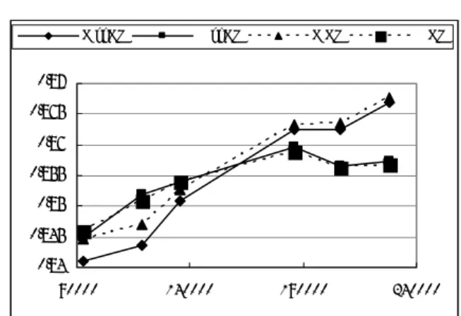
(7) Ent method, and the performance of MaxEnt is not worse than SVMs. Test data T N A M T N A M. Dep. Root Nivre, SVMs 86.95 92.08 80.28 86.99 87.52 92.71 76.67 85.41 Nivre, MaxEnt 87.39 89.61 81.06 83.98 87.56 91.50 77.87 82.05. Sent. 72.14 56.88 74.50 48.61 76.30 60.08 74.50 51.74. comes worse according to increasing the training data.. Dep. Root Sent. Yamada, SVMs 87.63 93.07 74.31 77.39 88.98 52.87 86.20 94.15 70.75 76.34 87.55 48.78 Yamada, MaxEnt 86.85 92.60 72.37 77.89 86.72 52.21 86.07 93.59 70.08 76.38 87.24 48.81. N noNP. Test data T N A M T N A M. Dep. Root Nivre, SVMs 87.07 83.87 80.88 77.10 87.61 84.16 77.20 72.60 Nivre, MaxEnt 87.32 89.61 81.21 83.98 87.63 91.61 78.21 82.13. Sent. 65.98 49.82 65.43 41.77 76.30 60.84 74.72 52.82. Table 6: The result of experiment 2 Figure 4 shows the result of experiment 3, namely the performance of using Nivre’s algorithm with the NP-chunker by increasing training data. There are two testing data shown in the figure (Newspaper and Magazine). Each testing data were tested with the NP-chunker or without. According to this result, method using the NPchunker doesn’t achieve higher accuracy. But we trust this is caused by the low performance of NP-chunker and the narrow definition of our base-NP. Alternatively, the figure shows that the best performance of different training data size is about 185,000 words. Although the accuracy of testing data “Newspaper” is improved by using more data size, the accuracy of “Magazine” be-. M NP. 0.87. 0.86 0.855 0.85 0.845 0.84 90000. Dep. Root Sent. Yamada, SVMs 87.67 86.32 70.24 79.02 72.5 46.23 86.67 83.12 63.31 77.33 71.11 42.22 Yamada, MaxEnt 86.86 92.60 72.73 78.87 86.59 54.77 86.18 93.59 70.64 77.09 87.21 50.42. N NP. 0.865. Table 5: The result of experiment 1 Table 6 shows the result of experiment 2. This experiment conducts for two algorithms with the NP-chunker. Comparing with Table 5, the performance does not jump up after using NPchunker. According to this result, it seems that we didn’t need to add the NP-chunker in our analyzer. This is because that the accuracy of our NP-chunker is 88.21 (Recall). There are many base-NP which cannot be extracted correctly. This is a major error source in our experiment.. M noNP. 140000. 190000. 240000. Figure 4: The result of experiment 3: the model with NP-chunker among the different training data sizes. 4. Discussion. This section shows error analysis on the experimental results.. 4.1. Base NP. The reason that we used the NP-chunker is that there are many nominal compounds in Chinese, especially in newspaper. For example: 國際/貨幣 / 基金會 (IMF), 太空 / 衛星 / 計畫 (satellite project)…etc. Most of nominal compounds are combined from two or three noun words. Therefore, when a long noun sequence – namely a nominal compound – was analyzed, our models tend to separate the sequence into two or three base-NPs. For instance: base-NP “行政院 /經濟 /建設 /委員會” is an organization name. Each word should depend on the last word “委員會”, but our analyzer separated this base-NP into two base-NPs: “行政院” and “經濟 /建設 /委員會”. Therefore, we should use the NP-chunker to avoid such errors. Although we used the NP-chunker in our analyzer, the result was not very good. Because the performance of NP-chunker is not perfect. Actually, the NP-chunker cannot extract 18% of the base-NPs correctly. The task of extracting baseNP is difficult. Alternatively, our definition of base-NP is too restricted. There are many baseNPs that include not only nouns but also other words. For example, the NP “今年(Nd)/一(Nd)/ 到(Ca)/ 十月(Nd)” cannot be extracted by our. 7 −97−.

(8) NP-chunker. We should extend the definition of base-NP and improve the performance of the NPchunker.. 4.2. PP Extraction. The structure of prepositional phrases is “prep. + NP”, “prep. +VP”, or “prep. +S”. It is difficult to identify the boundary of PP. Sometimes the preposition will make a long sentence. However, our analyzer tends to let the preposition governing a partial subtree of the full sentence. Some prepositions in Chinese are not only a preposition but also a predicate. For example, the preposition “在(in, at)” can be a simple prep.— “他(he)/在(at)/學校(school)/吃飯(eat lunch) (He ate lunch at school.)”. The preposition “在(at)” takes a PP (在/學校 at school). However, it can be also a predicate – “ 他 (he)/ 在 (stay at)/ 家 (home) He stays at home”. These properties of PP cause 15% of errors in our experiments. There are two ways to alleviate these problems. First, we should identify the predicate prepositions from corpus. These prepositions are obstacles to the machine learning of normal prepositions and should be regarded as a different POS. Second, if the analyzer can extract the element that dependent on a preposition (NP, VP, S, etc.), the performance will improve.. 4.3. Shift and Reduce. As described in Section 2.1, Nivre’s algorithm can resolve the ambiguity between of the action Shift and Left (in Yamada’s algorithm). The action Reduce needs the condition that the node n should have no more child in I. However, it is difficult to identify this condition. In some long sentences, the children of the focused node n may be at the end node of the sentence. Moreover, some non-local dependency will cause this kind of error. This caused 15 % of errors in our experiments.. 5. Conclusion and Future Work. In this paper, we presented a deterministic dependency structure analyzer for Chinese. This analyzer implements two algorithms with two machine learning methods, SVMs and MaxEnt. We compared the performance of the two models on a dependency tagged corpus derived from the CKIP Treebank corpus. The result shows that Nivre’s method can resolve some problems in Yamada’s method and the MaxEnt can obtain. good performance. Next, we tried to add an NPchunker in our model. Although the result of the NP-chunker experiment didn’t show significantly better performance, we discuss that using an NPchunker is necessary for Chinese dependency analyzing. Future work includes three parts. First, as discussed in Section 4, we should improve our NPchunker to resolve the NP extracting problem. We should also try to establish PP-chunker to identify PP. Second, the ambiguity between two actions – Shift and Reduce – should be resolved by long-distance dependency resolution model. Third, for applying to wide region of Chinese texts, we will evaluate our method on the Penn Chinese Treebank which contains articles from the newspapers in mainland China. References. Adam Berger, Stephen Della Pietra, and Vincent Della Pietra, 1996. A Maximum Entropy Approach to Natural Language Processing, Computational Linguistics, vol. 22, no. 1 Jason Baldridge, Tom Morton, and Gann Bierner, 2001, http://maxent.sourceforge.net/ Eugene Charniak, 2000. A Maximum-EntropyInspired Parser. In Proc. of NAACL2000, pages 132–139. Keh-Jiann Chen, Chin-Ching Luo, Zhao-Ming Gao, Ming-Chung Chang, Feng-Yi Chen, Chao-Jan Chen, 1999, The CKIP Tree-bank: Guidelines for Annotation, Presented at ATALA Workshop, Paris, June 18-19. Yuchang Cheng , Masayuki, Asahara and Yuji Matsumoto, 2004. Deterministic dependency structure analyzer for Chinese, IJCNLP 2004. Michael Collins, 1997. Three Generative, Lexicalised Models for Statistical Parsing. In Proc.of ACLEACL 1997, pages 16–23. Darroch, J. Ratcli , D. 1972. Generlized Iterative Scaling for Log-linear Models. In Annals of Mathematical Statistics, volume 43, Issue 5, pages 14701480 Ulrich. H.-G. Kreβel, 1998. Pairwise classification and support vector machines. In Advances in Kernel Methods, pages 255–268. The MIT Press. Taku Kudo, Yuji Matsumoto, 2002. Japanese Dependency Analyisis using Cascaded Chunking, CONLL 2002 Joakim Nivre, 2004. Incrementality in Deterministic Dependency Parsing. ACL-2004. Adwait Ratnaparkhi, 1999. Learning to parse natural language with maximum entropy models. Machine Learning, 34(1-3):151–175 Vladimir N. Vapnik, 1998. Statistical Learning Theory. A Wiley-Interscience Publication. Hiroyasu Yamada and Yuji Matsumoto, 2003. Statistical Dependency Analysis with Support Vector Machines, IWPT 2003.. 8 −98−.

(9)