Simultaneous testing of the mean vector and
the covariance matrix with two-step
monotone missing data
Miki Hosoya and Takashi Seo
(Received August 18, 2014; Revised November 15, 2014)
Abstract. In this paper, we consider the problem of simultaneous testing of the mean vector and the covariance matrix when the data have a two-step monotone pattern that is missing observations. We give the likelihood ratio test (LRT) statistic and propose an approximate upper percentile of the null distribution using linear interpolation based on an asymptotic expansion of the modified LRT statistic in the case of a complete data set. As another approach, we give the modified LRT statistics with a two-step monotone missing data pattern using the coefficient of the modified LRT statistic with complete data. Finally, we investigate the asymptotic behavior of the upper percentiles of these test statistics by Monte Carlo simulation.
AMS 2010 Mathematics Subject Classification. 62E20, 62H10.
Key words and phrases. Asymptotic expansion, linear interpolation, modified
likelihood ratio test statistic, two-step monotone missing data.
§1. Introduction
Let x1, x2, . . . , xN1 be distributed as the p-dimensional normal distribution
Np(µ, Σ) and x1,N1+1, x1,N1+2, . . . , x1N be distributed as the p1-dimensional normal distribution Np1(µ1, Σ11), where
µ = ( µ1 µ2 ) , Σ = ( Σ11 Σ12 Σ21 Σ22 ) .
We partition xj into a p1× 1 random vector and a p2× 1 random vector as xj = (x′1j, x′2j)′, where xij : pi× 1, i = 1, 2, j = 1, 2, . . . , N1.
Such a data set has two-step monotone missing data: x′11 x′21 .. . ... x′1N1 x′2N1 N1 x′1,N 1+1 ∗ · · · ∗ .. . ... ... x′1N ∗ · · · ∗ N2 | {z } p1 | {z } p2 ,
where N = N1 + N2, p = p1 + p2, N1 > p, and “∗” indicates a missing
observation.
Missing data is an important problem in statistical data analyses. A variety of statistical procedures to deal with missing data have been developed by many authors, including Anderson (1957), Bhargava (1962), McLachlan and Krishnan (1997), and Little and Rubin (2002). For a general missing pattern, Srivastava (1985) discussed the LRT for mean vectors in one-sample and two-sample problems. Seo and Srivastava (2000) derived a test of equality of means and the simultaneous confidence intervals for the monotone missing data in a one-sample problem. Anderson (1957) developed an approach to derive the MLEs of the mean vector and the covariance matrix by solving the likelihood equations for monotone missing data with several missing patterns. Anderson and Olkin (1985) derived the MLEs for two-step monotone missing data in a one-sample problem. For the related discussion of the MLEs in cases of general
k-step monotone missing data, see Jinadasa and Tracy (1992) and Kanda and
Fujikoshi (1998).
Further, by the use of the MLEs of the mean vector and the covariance matrix, the LRT statistic and Hotelling’s T2-type statistic for tests of mean
vectors with two or three-step monotone missing data has been discussed by Krishnamoorthy and Pannala (1999), Chang and Richards (2009), Seko et al. (2012), and Yagi and Seo (2014), among others. The problem of simultaneous testing of the mean and the variance under univariate and non-missing nor-mality has been discussed by Choudhari et al. (2001) and Zhang et al. (2012). For non-missing and multivariate normality, Davis (1971) gave the modified LRT statistic (see Muirhead (1982) and Srivastava (2002)). In this paper, the LRT and modified LRT statistics are given under multivariate normality with a two-step monotone missing data pattern. Further, we assume that the data are missing completely at random (MCAR), see Hao and Krishnamoorthy (2001), and Little and Rubin (2002).
The remainder of this paper is organized as follows. In Section 2, we con-sider the case in which the missing observations are of the two-step monotone
type and provide an LRT statistic for the simultaneous testing of the mean vector and the covariance matrix. In Section 3, an approximation to the up-per up-percentile of the LRT statistic and the modified LRT statistics are given. Finally, in Section 4, the accuracy of the approximation and the asymptotic behavior of modified statistics are investigated by Monte Carlo simulation.
§2. Likelihood ratio test statistic
In order to derive the LRT statistic of the simultaneous testing of the mean vector and the covariance matrix in the case of a two-step monotone missing data pattern, we present their MLEs, which are given by
bµ = ( bµ1 bµ2 ) = N1(N1x(1)1+ N2x(2)) x(1)2− bΣ21bΣ−111(x(1)1− bµ1) , (2.1) bΣ = ( bΣ11 bΣ12 bΣ21 bΣ22 ) (2.2) = 1 N(W(1)11+ W(2)) bΣ11W −1 (1)11W(1)12 W(1)21W(1)11−1 bΣ11 1 N1 W(1)22·1+ bΣ21bΣ−111bΣ12 , where x(1) = ( x(1)1 x(1)2 ) , x(1)1= 1 N1 N1 ∑ j=1 x1j, x(1)2= 1 N1 N1 ∑ j=1 x2j, x(2) = 1 N2 N ∑ j=N1+1 x1j, and W(1)= ( W(1)11 W(1)12 W(1)21 W(1)22 ) = N1 ∑ j=1 (xj− x(1))(xj− x(1))′, W(2)= N ∑ j=N1+1 (x1j − x(2))(x1j− x(2))′+ N1N2 N (x(1)1− x(2))(x(1)1− x(2)) ′, W(1)22·1= W(1)22− W(1)21W(1)11−1 W(1)12 .
These results follow from the results in Anderson and Olkin (1985) and Kanda and Fujikoshi (1998).
In the derivation, we use the following transformed parameters (η, ∆) : η = ( η1 η2 ) = ( µ1 µ2− ∆21µ1 ) , ∆ = ( ∆11 ∆12 ∆21 ∆22 ) = ( Σ11 Σ−111Σ12 Σ21Σ−111 Σ22·1 ) ,
where Σ22·1 = Σ22− Σ21Σ−111Σ12. We note that (η, ∆) are in one-to-one
cor-respondence to (µ, Σ). After multiplying the observation vector xj by the
transformation matrix A = ( Ip1 O −∆21 Ip2 )
on the left side, the log likelihood function is derived, and the results can then be obtained by differentiation.
We consider the following hypothesis test when the data set is of a two-step monotone pattern.
H0 : µ = µ0, Σ = Σ0 vs. H1: not H0.
(2.3)
Without loss of generality, we can assume that µ = 0 and Σ = Ip. Then, from
the MLEs in (2.1) and (2.2), we obtain the following theorem.
Theorem 2.1. Suppose that the data have a two-step monotone pattern that
is missing observations and that λ1 is the likelihood ratio (LR) in the case of the two-step monotone missing data. Then, the LR of the hypothesis test (2.3) is given by λ1=|bΣ11| N 2|bΣ22·1|N12 etr −1 2 N ∑ j=1 x1jx′1j etr −1 2 N1 ∑ j=1 x2jx′2j exp ( −1 2N p1 ) exp ( −1 2N1p2 ) .
Further, the LR can be expressed as λ1 = ( e N )1 2N p1 |W(1)11+ W(2)| 1 2N × etr [ −1 2 { W(1)11+W(2)+ 1 N(N1x(1)1+N2x(2))(N1x(1)1+N2x(2)) ′}] × ( e N1 )1 2N1p2 |W(1)22·1| 1 2N1etr { −1 2(W(1)22+ N1x(1)2x ′ (1)2) } .
The result in Theorem 2.1 coincides with the result in Hao and Krishnamoor-thy (2001). We note that under H0,−2 log λ1 is asymptotically distributed as
a χ2 distribution with f = p(p + 3)/2 degrees of freedom when N1, N → ∞
with N1/N → δ ∈ (0, 1]. However, when the sample size is not large, the χ2
distribution is not a good approximation to the upper percentile of−2 log λ1.
Further, it is not easy to find the exact distribution of the LRT statistic
−2 log λ1. In the next section, we give an approximate upper percentile of −2 log λ1 and propose modified LRT statistics whose upper percentile is close
to that of the χ2 distribution even for small samples.
§3. The modified LRT statistics and an approximate upper
percentile of the LRT statistic
In this section, we propose an approximate upper percentile of the null distri-bution of −2 log λ1 using linear interpolation based on an asymptotic
expan-sion of the modified LRT statistic in the case of a complete data set. Further, as another approach, we give the modified LRT statistics using the coefficient of the modified LRT statistic for the complete data.
3.1. Modified coefficient approximation procedure
We first consider the LR in the case of a complete data set. Let x1, x2, . . . , xN
∼ Np(µ, Σ), and let λc,N be the LR for the complete data set. Then, the LR is given by λc,N = (e N )N p 2 |V |N 2etr { −1 2(V + N x x ′)}, where x = 1 N N ∑ i=1 xi, V = N ∑ i=1 (xi− x)(xi− x)′.
Further, the modified LRT statistic is given by−2ρc,Nlog λc,N, where ρc,N = 1− (2p2+ 9p + 11)/{6N(p + 3)}, and its cumulative distribution function can be expanded as Pr(−2ρc,Nlog λc,N ≤ x) = Gf(x)+ γ M2 {Gf +4(x)−Gf(x)}+O(M −3), (3.1) where M = ρc,NN, γ = p 288(p + 3)(2p 4+ 18p3+ 49p2+ 36p− 13),
and Gf(x) and Gf +4(x) are the cumulative distribution functions of the χ2
distribution with f (= p(p + 3)/2) and f + 4 degrees of freedoms, respectively. This result was derived by Davis (1971) (see Muirhead ((1982), p. 370) and Srivastava ((2002), p. 494)). This means that if the χ2 distribution is used as an approximation to the distribution of −2ρc,Nlog λc,N, the error involved is not of order M−1 but of order M−2.
If we denote the coefficients of the modified LRT statistics in the case of complete data sets N and N1 by ρc,N and ρc,N1, respectively, then it may be noted that ρmiss is between ρc,N and ρc,N1, where ρmiss is the coefficient of the modified LRT statistic −2ρmisslog λ1. From the linear interpolation, we
propose an approximation to the modified LRT statistic in the case of two-step monotone missing data. Calculating the approximate coefficient ρL =
(p1ρc,N + p2ρc,N1)/p, we can obtain an approximate modified LRT statistic
−2ρLlog λ1, where ρL= 1− 1 N ( 1 +N2p2 N1p ) 2p2+ 9p + 11 6(p + 3) .
3.2. Asymptotic expansion approximation procedure
In this subsection, we give an approximate upper percentile of−2 log λ1 when
the data have a two-step monotone pattern that is missing observations. First, in the case of a complete data set, we obtain the following lemma.
Lemma 3.1. Suppose that x1, x2, . . . , xN are distributed as Np(µ, Σ). Then,
under the null hypothesis H0 in (2.3), the upper percentile of the modified LRT statistic,−2ρc,Nlog λc,N, can be expanded as
qMLR·c(α) = χ2f(α) + 1 M2 2γ f (f + 2)χ 2 f(α) { χ2f(α) + f + 2}+ o(M−2), where M = ρc,NN, ρc,N = 1− 2p2+ 9p + 11 6N (p + 3) , f = 1 2p(p + 3), and χ2
f(α) is the upper percentile of the χ2 distribution with f degrees of
free-dom.
Proof. Putting the upper percentile of −2ρc,Nlog λc,N with
qMLR·c(α) = χ2f(α) +
1
where h is a constant, we have 1− α = Gf(qMLR·c(α))− gf(χ2f(α)) 1 M2h + o(M −2), (3.2)
where Gf(x) and gf(x) are, respectively, the cumulative distribution function
and the density function of the χ2 distribution with f degrees of freedom. On the other hand, from (3.1), we can write
1− α = Pr {−2ρc,Nlog λc,N ≤ qMLR·c(α)} = Gf(qMLR·c(α)) + γ M2{Gf +4(qMLR·c(α))− Gf(qMLR·c(α))} (3.3) + o(M−2).
Therefore, using Gf +2j(x) = −2gf +2j(x) + Gf +2(j−1)(x), j = 0, 1, 2 and
comparing (3.2) with (3.3), we obtain
h = 2γ f (f + 2)χ 2 f(α) { χ2f(α) + f + 2}+ o(M−2).
From Lemma 3.1 and M−2 = N−2+ O(N−3), we can expand the upper percentile of−2 log λc,N as qLR·c(α) = χ 2 f(α) + ν Nχ 2 f(α) + 1 N2χ 2 f(α) { ν2+2γ f + 2γ f (f + 2)χ 2 f(α) } +o(N−2), where ν = 2p 2+ 9p + 11 6(p + 3) .
From the linear interpolation, letting qLR·m(α) be the upper percentile of
−2 log λ1, an approximate upper percentile of−2 log λ1 can be obtained as qLR∗ ·m(α) = χ2f(α) + 1 N ( p1+ 1 c1 p2 ) ν pχ 2 f(α) + 1 N2 ( p1+ 1 c21p2 )χ2 f(α) p { ν2+2γ f + 2γ f (f + 2)χ 2 f(α) } + o(N−2), where c1 = N1/N.
3.3. The LRT statistic’s decomposition procedure
In this section, we give other modified LRT statistics by the decomposition of
λ1. We first consider the following test problem for Σ.
H01: Σ = Σ0= I vs. H11: Σ̸= I.
Hao and Krishnamoorthy (2001) derived the modified LRT statistic λ∗Σ in the case of two-step monotone missing data, which is given by
λ∗Σ= (e n )1 2np1 W(1)11+ W(2) 1 2nexp { −1 2tr(W(1)11+ W(2)) } × ( e n1 )1 2n1p2 W(1)22·1 1 2n1exp { −1 2trW(1)22·1 } × exp { −1 2tr(W(1)21W −1 (1)11W(1)12) } ,
where n = N− 1, n1= N1− p1− 1. We note that the modified LRT statistic −2 log λ∗
Σ is an unbiased test statistic (see Hao and Krishnamoorthy (2001)
and Chang and Richards (2010)). Further, after modifying and rearranging some terms, Hao and Krishnamoorthy (2001) expressed the modified LR for
H0 in (2.3) as λ∗Σω1ω2, where ω1 = exp { − 1 2N(N1x(1)1+ N2x(2)) ′(N 1x(1)1+ N2x(2)) } , ω2 = exp { −1 2N1x ′ (1)2x(1)2 } . If we denote ω3= (e N )1 2N p1 |W(1)11+ W(2)| 1 2Nexp { −1 2tr(W(1)11+ W(2)) } , ω4= ( e N1 )1 2N1p2 |W(1)22·1| 1 2N1exp { −1 2trW(1)22·1 } , ω5= exp { −1 2tr(W(1)21W −1 (1)11W(1)12) } , we can express λ1 = ∏5
i=1ωi. Since ω1ω3 and ω2ω4 are of the form of LR
for H0 under non-missing normality, we can give the modified LRT statistics, −2ρ13log ω1ω3 and −2ρ24log ω2ω4, respectively, where
ρ13= 1− 2p21+ 9p1+ 11 6N (p1+ 3) , ρ24= 1− 2p22+ 9p2+ 11 6N1(p2+ 3) .
Thus, we propose a new modified LRT statistic given by−2 log τ, where τ = (ω1ω3)ρ13(ω2ω4)ρ24ω5 . In addition, we denote ω∗3 = (e n )1 2np1 |W(1)11+ W(2)| 1 2nexp { −1 2tr(W(1)11+ W(2)) } , ω∗4 = ( e n1 )1 2n1p2 |W(1)22·1| 1 2n1exp { −1 2trW(1)22·1 } .
Then, since ω3∗ and ω∗4 are of the form of LR for H01 under non-missing
nor-mality, we can propose the modified LRT statistic −2 log φ∗, where
φ∗= ω1ω2(ω∗3)ρ ∗ 3(ω∗ 4)ρ ∗ 4ω 5 and ρ∗3 = 1−2p 2 1+ 3p1− 1 6n(p1+ 1) , ρ∗4 = 1−2p 2 2+ 3p2− 1 6n1(p2+ 1) . §4. Simulation studies
We evaluate the accuracy and the asymptotic behaviors of the χ2 approxima-tions by Monte Carlo simulation (106 runs).
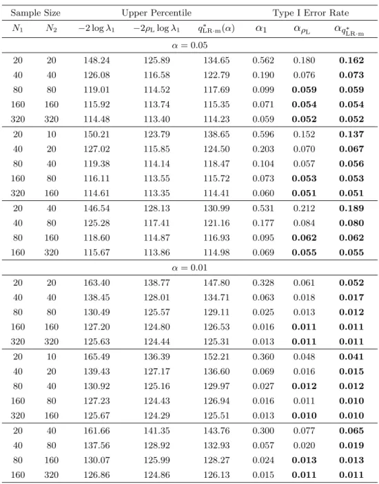
In Table 1, we provide the simulated upper 100α percentiles of −2 log λ1
and −2ρLlog λ1 and the approximate upper percentiles of −2 log λ1, that is, qLR∗ ·m(α) for (p1, p2) = (8, 4); α = 0.05, 0.01; and for the following three cases
of (N1, N2), (N1, N2) = (m, m), m = 20, 40, 80, 160, 320, (2m, m), m = 10, 20, 40, 80, 160, (m, 2m), m = 20, 40, 80, 160.
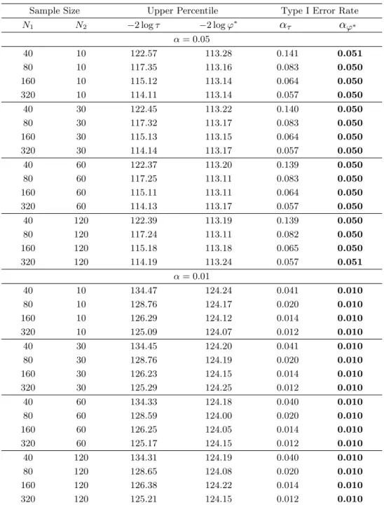
In Table 2, we provide the same upper percentiles as those given in Table 1 for (p1, p2) = (8, 4); α = 0.05, 0.01; (N1, N2) = (m1, m2), m1 = 40, 80, 160, 320, m2 = 10, 30, 60, 120, where the sets of (N1, N2) are combinations of m1 and m2.
It may be noted from Tables 1 and 2 that the simulated values are closer to the upper percentile of the χ2 distribution when the sample size becomes
large. In addition, it can be seen from both tables that the upper percentile of
−2ρLlog λ1 is considerably better than that of−2 log λ1 even for small sample
sizes. Further, Tables 1 and 2 list the actual type I error rates for the upper percentiles of −2 log λ1 and −2ρLlog λ1 as well as qLR∗ ·m(α), which are given
by α1= Pr { −2 log λ1 > χ2f(α) } , αρL= Pr { −2ρLlog λ1 > χ2f(α) } , and αqLR∗ ·m = Pr{−2 log λ1 > qLR∗ ·m(α)} ,
respectively. It appears from the simulated results that the approximate value
qLR∗ ·m(α) based on the asymptotic expansion is good for all cases, even when
N1 < N2. Therefore, it can be concluded that our approximation procedures
are very accurate for most of the cases.
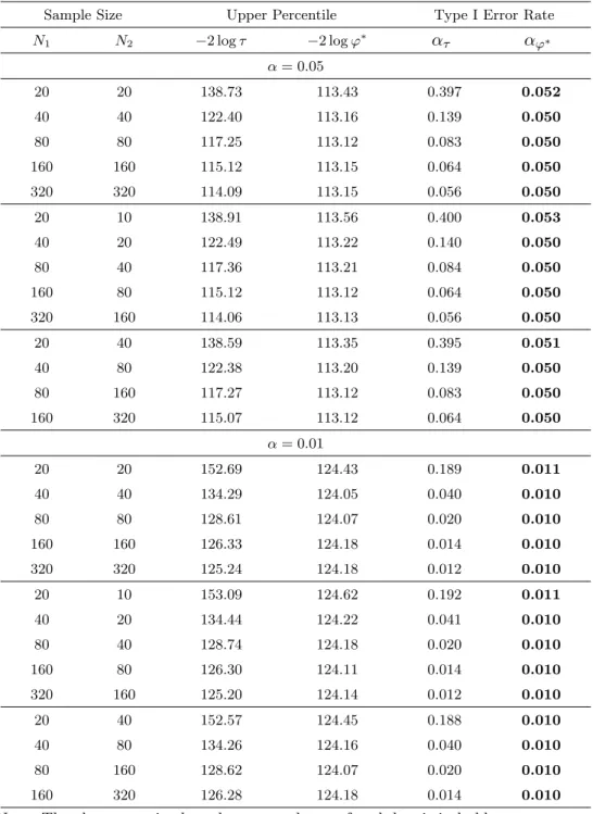
In Tables 3 and 4, we provide the simulated upper percentiles of −2 log τ and −2 log φ∗ for the same cases as those in Tables 1 and 2. It may also be noted that the upper percentiles of −2 log φ∗ are considerably good even for small sample sizes. Tables 3 and 4 list the actual type I error rates for the upper percentiles of−2 log τ and −2 log φ∗, which are given by
ατ = Pr { −2 log τ > χ2 f(α) } and αφ∗ = Pr { −2 log φ∗ > χ2 f(α) } ,
respectively. The results for actual type I error rates also show that our modified LRT statistic−2 log φ∗ yields considerably good χ2 approximations
for cases in which the sample size is small.
In conclusion, we have developed the approximate upper percentiles of the LRT statistic −2 log λ1 and some modified LRT statistics for simultaneous
testing of the mean vector and the covariance matrix for the case of two-step monotone missing data. The null distribution of the modified LRT statistic
−2 log φ∗ proposed in this paper has considerably good approximation to the
Table 1: The simulated values for−2 log λ1 and −2ρLlog λ1, and the
approx-imate value for −2 log λ1, and the type I error rates when (p1, p2) = (8, 4)
Sample Size Upper Percentile Type I Error Rate
N1 N2 −2 log λ1 −2ρLlog λ1 qLR∗ ·m(α) α1 αρL αqLR∗ ·m α = 0.05 20 20 148.24 125.89 134.65 0.562 0.180 0.162 40 40 126.08 116.58 122.79 0.190 0.076 0.073 80 80 119.01 114.52 117.69 0.099 0.059 0.059 160 160 115.92 113.74 115.35 0.071 0.054 0.054 320 320 114.48 113.40 114.23 0.059 0.052 0.052 20 10 150.21 123.79 138.65 0.596 0.152 0.137 40 20 127.02 115.85 124.50 0.203 0.070 0.067 80 40 119.38 114.14 118.47 0.104 0.057 0.056 160 80 116.11 113.55 115.72 0.073 0.053 0.053 320 160 114.61 113.35 114.41 0.060 0.051 0.051 20 40 146.54 128.13 130.99 0.531 0.212 0.189 40 80 125.28 117.41 121.16 0.177 0.084 0.080 80 160 118.60 114.87 116.93 0.095 0.062 0.062 160 320 115.67 113.86 114.98 0.069 0.055 0.055 α = 0.01 20 20 163.40 138.77 147.80 0.328 0.061 0.052 40 40 138.45 128.01 134.71 0.063 0.018 0.017 80 80 130.49 125.57 129.11 0.025 0.013 0.012 160 160 127.20 124.80 126.53 0.016 0.011 0.011 320 320 125.63 124.44 125.31 0.013 0.011 0.011 20 10 165.49 136.39 152.21 0.360 0.048 0.041 40 20 139.43 127.17 136.60 0.069 0.016 0.015 80 40 130.92 125.16 129.97 0.027 0.012 0.012 160 80 127.23 124.43 126.94 0.016 0.011 0.010 320 160 125.67 124.29 125.51 0.013 0.010 0.010 20 40 161.66 141.35 143.76 0.300 0.077 0.065 40 80 137.56 128.92 132.93 0.057 0.020 0.019 80 160 130.07 125.99 128.27 0.024 0.013 0.013 160 320 126.86 124.86 126.13 0.015 0.011 0.011
Note. The closest to α in the values α1, αρL, and αq∗
LR·m of each low is in bold.
χ2
Table 2: The simulated values for−2 log λ1 and −2ρLlog λ1, and the
approx-imate value for −2 log λ1, and the type I error rates when (p1, p2) = (8, 4)
Sample Size Upper Percentile Type I Error Rate
N1 N2 −2 log λ1 −2ρLlog λ1 qLR∗ ·m(α) α1 αρL αqLR∗ ·m α = 0.05 40 10 127.69 115.18 125.92 0.214 0.064 0.061 80 10 119.81 113.54 119.55 0.109 0.053 0.052 160 10 116.45 113.29 116.35 0.075 0.051 0.051 320 10 114.78 113.19 114.75 0.061 0.050 0.050 40 30 126.47 116.26 123.51 0.196 0.074 0.070 80 30 119.49 113.97 118.76 0.105 0.056 0.055 160 30 116.28 113.34 116.12 0.074 0.051 0.051 320 30 114.70 113.17 114.68 0.061 0.050 0.050 40 60 125.61 117.09 121.80 0.182 0.081 0.077 80 60 119.14 114.33 118.02 0.101 0.058 0.057 160 60 116.16 113.48 115.86 0.073 0.052 0.052 320 60 114.70 113.25 114.60 0.061 0.051 0.051 40 120 124.90 117.84 120.38 0.172 0.088 0.084 80 120 118.72 114.70 117.23 0.097 0.061 0.060 160 120 115.95 113.61 115.51 0.071 0.053 0.053 320 120 114.61 113.29 114.48 0.061 0.051 0.051 α = 0.01 40 10 140.21 126.48 138.17 0.075 0.014 0.013 80 10 131.45 124.57 131.15 0.029 0.011 0.010 160 10 127.73 124.26 127.63 0.017 0.010 0.010 320 10 125.85 124.10 125.87 0.013 0.010 0.010 40 30 138.67 127.47 135.51 0.066 0.017 0.016 80 30 131.24 125.17 130.28 0.028 0.012 0.012 160 30 127.53 124.31 127.38 0.017 0.010 0.010 320 30 125.76 124.09 125.81 0.013 0.010 0.010 40 60 137.82 128.47 133.63 0.060 0.019 0.018 80 60 130.74 125.46 129.47 0.026 0.012 0.012 160 60 127.43 124.48 127.09 0.016 0.011 0.011 320 60 125.79 124.20 125.72 0.013 0.010 0.010 40 120 137.08 129.34 132.07 0.055 0.021 0.020 80 120 130.35 125.93 128.60 0.024 0.013 0.013 160 120 127.22 124.65 126.71 0.016 0.011 0.011 320 120 125.60 124.15 125.58 0.013 0.010 0.010
Note. The closest to α in the values α1, αρL, and αq∗
LR·m of each low is in bold.
χ2
f(0.05) = 113.145, χ
2
Table 3: The simulated values for−2 log τ and −2 log φ∗, and the type I error rates when (p1, p2) = (8, 4)
Sample Size Upper Percentile Type I Error Rate
N1 N2 −2 log τ −2 log φ∗ ατ αφ∗ α = 0.05 20 20 138.73 113.43 0.397 0.052 40 40 122.40 113.16 0.139 0.050 80 80 117.25 113.12 0.083 0.050 160 160 115.12 113.15 0.064 0.050 320 320 114.09 113.15 0.056 0.050 20 10 138.91 113.56 0.400 0.053 40 20 122.49 113.22 0.140 0.050 80 40 117.36 113.21 0.084 0.050 160 80 115.12 113.12 0.064 0.050 320 160 114.06 113.13 0.056 0.050 20 40 138.59 113.35 0.395 0.051 40 80 122.38 113.20 0.139 0.050 80 160 117.27 113.12 0.083 0.050 160 320 115.07 113.12 0.064 0.050 α = 0.01 20 20 152.69 124.43 0.189 0.011 40 40 134.29 124.05 0.040 0.010 80 80 128.61 124.07 0.020 0.010 160 160 126.33 124.18 0.014 0.010 320 320 125.24 124.18 0.012 0.010 20 10 153.09 124.62 0.192 0.011 40 20 134.44 124.22 0.041 0.010 80 40 128.74 124.18 0.020 0.010 160 80 126.30 124.11 0.014 0.010 320 160 125.20 124.14 0.012 0.010 20 40 152.57 124.45 0.188 0.010 40 80 134.26 124.16 0.040 0.010 80 160 128.62 124.07 0.020 0.010 160 320 126.28 124.18 0.014 0.010
Note. The closer to α in the values ατ and αφ∗ of each low is in bold.
Table 4: The simulated values for−2 log τ and −2 log φ∗, and the type I error rates when (p1, p2) = (8, 4)
Sample Size Upper Percentile Type I Error Rate
N1 N2 −2 log τ −2 log φ∗ ατ αφ∗ α = 0.05 40 10 122.57 113.28 0.141 0.051 80 10 117.35 113.16 0.083 0.050 160 10 115.12 113.14 0.064 0.050 320 10 114.11 113.14 0.057 0.050 40 30 122.45 113.22 0.140 0.050 80 30 117.32 113.17 0.083 0.050 160 30 115.13 113.15 0.064 0.050 320 30 114.14 113.17 0.057 0.050 40 60 122.37 113.20 0.139 0.050 80 60 117.25 113.11 0.083 0.050 160 60 115.11 113.11 0.064 0.050 320 60 114.13 113.17 0.057 0.050 40 120 122.39 113.19 0.139 0.050 80 120 117.24 113.11 0.082 0.050 160 120 115.18 113.18 0.065 0.050 320 120 114.19 113.24 0.057 0.051 α = 0.01 40 10 134.47 124.24 0.041 0.010 80 10 128.76 124.17 0.020 0.010 160 10 126.29 124.12 0.014 0.010 320 10 125.09 124.07 0.012 0.010 40 30 134.45 124.20 0.041 0.010 80 30 128.76 124.19 0.020 0.010 160 30 126.23 124.15 0.014 0.010 320 30 125.29 124.25 0.012 0.010 40 60 134.33 124.18 0.040 0.010 80 60 128.59 124.00 0.020 0.010 160 60 126.25 124.05 0.014 0.010 320 60 125.17 124.15 0.012 0.010 40 120 134.31 124.19 0.040 0.010 80 120 128.65 124.08 0.020 0.010 160 120 126.38 124.22 0.014 0.010 320 120 125.21 124.15 0.012 0.010
Note. The closer to α in the values ατ and αφ∗ of each low is in bold.
χ2
f(0.05) = 113.145, χ
2
Acknowledgments
The authors would like to thank the referee for helpful comments and sug-gestions. Second author’s research was in part supported by Grant-in-Aid for Scientific Research (C) (26330050).
References
[1] Anderson, T. W. (1957). Maximum likelihood estimates for a multivariate normal distribution when some observations are missing, J. Amer. Statist. Assoc., 52, 200–203.
[2] Anderson, T. W. and Olkin, I. (1985). Maximum-likelihood estimation of the parameters of a multivariate normal distribution, Linear Algebra Appl., 70, 147– 171.
[3] Bhargava, R. (1962). Multivariate tests of hypotheses with incomplete data, Technical Report No.3, Applied Mathematics and Statistics Laboratories, Stan-ford University, StanStan-ford, California.
[4] Chang, W. -Y. and Richards, D. St. P. (2009). Finite-sample inference with monotone incomplete multivariate normal data, I, J. Multivariate Anal., 100, 1883–1899.
[5] Chang, W. -Y. and Richards, D. St. P. (2010). Finite-sample inference with monotone incomplete multivariate normal data, II, J. Multivariate Anal., 101, 603–620.
[6] Choudhari, P., Kundu, D. and Misra, N. (2001). Likelihood ratio test for simul-taneous testing of the mean and the variance of a normal distribution, J. Statist. Comuput. Simul., 71, 313–333.
[7] Davis, A. W. (1971). Percentile approximations for a class of likelihood ratio criteria, Biometrika, 58, 349–356.
[8] Hao, J. and Krishnamoorthy, K. (2001). Inferences on a normal covariance matrix and generalized variance with monotone missing data, J. Multivariate Anal., 78, 62–82.
[9] Jinadasa, K. G. and Tracy, D. S. (1992). Maximum likelihood estimation for multivariate normal distribution with monotone sample, Comm. Statist. Theory Methods, 21, 41–50.
[10] Kanda, T. and Fujikoshi, Y. (1998). Some basic properties of the MLE’s for a multivariate normal distribution with monotone missing data, Amer. J. Math. Management Sci., 18, 161–190.
[11] Krishnamoorthy, K. and Pannala, M. K. (1999). Confidence estimation of a normal mean vector with incomplete data, Canad. J. Statist., 27, 395–407.
[12] Little, R. J. and Rubin, D. B. (2002). Statistical Analysis with Missing Data, 2nd ed., Hoboken, NJ: Wiley.
[13] McLachlan, J. G. and Krishnan, T. (1997). The EM Algorithm and Extensions, New York, NY: Wiley.
[14] Muirhead, R. J. (1982). Aspects of Multivariate Statistical Theory, New York, NY: Wiley.
[15] Seo, T. and Srivastava, M. S. (2000). Testing equality of means and simultaneous confidence intervals in repeated measures with missing data, Biometrical J., 42, 981–993.
[16] Seko, N., Yamazaki, A. and Seo, T. (2012). Tests for mean vector with two-step monotone missing data, SUT J. Math., 48, 13–36.
[17] Srivastava, M. S. (1985). Multivariate data with missing observations, Comm. Statist. Theory Methods, 14, 775–792.
[18] Srivastava, M. S. (2002). Methods of Multivariate Statistics, New York, NY: Wiley.
[19] Yagi, A. and Seo, T. (2014). A test for mean vector and simultaneous confidence intervals with three-step monotone missing data, Amer. J. Math. Management Sci., 33, 161–175.
[20] Zhang, L., Xu, X. and Chen, G. (2012). The exact likelihood ratio test for equality of two normal populations, Amer. Statist., 66, 180–184.
Miki Hosoya
Department of Mathematical Information Science Tokyo University of Science
1-3, Kagurazaka, Shinjuku-ku, Tokyo 162-8601, Japan
E-mail : [email protected]
Takashi Seo
Department of Mathematical Information Science Tokyo University of Science
1-3, Kagurazaka, Shinjuku-ku, Tokyo 162-8601, Japan