著者
REIKA NOMURA
学位授与機関
Tohoku University
学位授与番号
11301甲第19295号
A DISSERTATION
SUBMITTED TO THE DEPARTMENT OF CIVIL ENGINEERING AND THE COMMITTEE ON GRADUATE STUDIES
OF TOHOKU UNIVERSITY
IN PARTIAL FULFILLMENT OF THE REQUIREMENTS FOR THE DEGREE OF DOCTOR OF ENGINEERING
REIKA NOMURA January 2020
The main purpose of this dissertation is to propose reliable evaluation schemes of the effects of trees’ presence in two-dimensional (2D) shallow water flows by conducting three-dimensional (3D) direct numerical flow simulations along the lines of the multi-scale modeling. We develop two types of multimulti-scale evaluation schemes based on the idea that the macro-scale shallow water flow can be equivalent to the homogenized micro-scale 3D flow in terms of energy or momentum balance. Throughout this dis-sertation, the stabilized finite element method (SUPG/PSPG) is used to solve both the 2D and 3D flow problems and Phase-Field method is employed to capture the free surfaces in the 3D direct flow simulations. We first establish two spatial-scales, and micro-scale, to define the microscopic domain to be a part of a macro-scale field. Then, the micro-macro-scale flow domain is identified with the local test domain (LTD), where a series of Navier-Stokes flow simulations is conducted to evaluate the macro-scale flow characteristics. We carry out a case study to validate the 3D flow simulations inside the established LTD consisting of 26 miniature rigid tree models and then confirm that our detailed branch modeling is adequate for the evaluation of the resistance of trees. With the LTD, we evaluate the macroscopic flow character-istics reflecting the effects of trees in shallow water flow by 3D direct numerical flow simulations. More specifically, the information obtained from the detailed flow simu-lations at the micro-scale is used to evaluate a parameter representing trees’ presence that enables us to carry out efficient macro-scale flow simulations in practical situa-tions. In this study, we refer to this procedure as ‘numerical flow test(s)’. Appropriate inflow and boundary conditions are provided to evaluate the effects of the complex shape of rigid trees models. In the two proposed multiscale evaluation process, either
characteristics. In the first type, we consider the equilibrium of the energy dissipations on the micro- and macro-scales. In this evaluation procedure, the microscopic energy dissipation caused by the flow through the trees arranged inside the LTD is thought to be equal to the work rate of the trees’ resistance in the macro-scale flow. Based on this theoretical development, the roughness coefficients are evaluated as macroscopic flow characteristics, which are used in the shear stress term of the 2D shallow water equation. Several macro-scale flow analyses are carried out to confirm that the en-ergy dissipation evaluated with the macroscopic roughness coefficients is comparable with the microscopic flow-induced energy dissipation. Also, the flow surface profile obtained by the 2D flow simulation reasonably agrees with that of the 3D numerical flow test. The second multiscale evaluation method proposed in this study focuses on the balance of the momentum losses on the micro- and macro-scales. This evaluation scheme is based on the idea that the total momentum loss supposed to be measured in the macro scale-flow is approximately equivalent to the dynamic pressure loss mea-sured in the LTD. The results of numerical flow tests enable us to equate these micro and macroscopic quantities to provide the drag term in the macro scale-flow equation with momentum loss parameter. These discrete values of the macroscopic momen-tum loss-parameters are used to construct the response surface based on the surrogate modeling; that is, the response surface is a surrogate model of the drag coefficient as a function of the inflow conditions for the LTD. The results of the macroscopic flow simulations with this surrogate model show reasonable agreements with those of the 3D microscopic flow simulations. In addition to the comparison of the flow states, we investigate the computational costs of the macro-scale flow simulations to confirm the efficiency of the proposed approach. Finally, the macro-scale flow characteris-tics, which are obtained from the two multiscale evaluation schemes, are examined through several unsteady-state flow simulations. Taking a dam-break problem, whose unsteadiness is supposed to be similar to the actual phenomena such as tsunami, as an example problem, we carry out the macroscopic flow simulations with the 2D shallow water equation incorporated with either the roughness coefficients or the surrogate
the proposed multiscale evaluation schemes and afford an insight into the significance of the inertial effects.
I would like to express my sincere gratitude to my supervisor Prof.Kenjiro Terada for all his supports. This work would not be accomplished without him. I am also thankful to the members of my dissertation committee: Dr. Anawat Suppasri, Prof. Shunichi Koshimura and Dr. Shuji Moriguchi for generously offering their time, com-ments and guidance throughout the review of this document. Thanks also to Dr. Shinsuke Takase for useful CFD codes, great mentorship, and encouragements. I also appreciate Prof. Takashi Kyoya and Prof. Randall J. LeVeque at the University of Washington for their valuable advice and comments, and former Prof. Kenjiro Hayashi at National Defence Academy of Japan for providing his hydraulic experi-mental data.
Some part of this work has been accomplished thanks to the funding from the following institution or academic program: Inter-Graduate School Doctoral Degree Program on Science for Global Safety (G-Safety program), Grant-in-Aid for JSPS Fellows (17J05235).
I also express my appreciation for the people whose supports were essential. Dr. Rumi Matsuzaki always made me feel confident and supported me to double-major in civil engineering and G-Safety leading program. I never forget Yashuko Uemura-sensei has provided me valuable lectures on academic writing and has taught me to be a witted global person. Special thanks to members who used to be pupils at Tohoku University together: F.Makinoshima, I.Tachibana, S.Nishi and T.Kotani for their technical supports to python/Fortran coding. 最後に,私の能力を常に信じ, 学業を支えてくれた父と母,兄そして両祖父母に感謝します.
Abstract iii
Acknowledgments vi
1 Introduction 1
1.1 On the global need for natural disaster mitigation . . . 1
1.2 Overview of ecosystem-based disaster mitigation . . . 2
1.3 Previous research on tsunami mitication forest . . . 5
1.4 Purpose and outline . . . 9
2 Multiscale modeling of flow through trees 13 2.1 Introduction . . . 13
2.2 Spatial scale separation . . . 13
2.2.1 Shallow water equation for 2D macroscopic flow . . . 14
2.2.2 Navier-Stokes equation for 3D microscopic flow . . . 16
2.3 Multiscale modeling based on numerical flow tests . . . 18
2.3.1 Procedure of numerical flow tests . . . 18
2.3.2 Local test domain . . . 18
2.3.3 Condition for numerical flow tests . . . 20
2.4 Validation analysis . . . 22
2.4.1 LTD with rigid trees models . . . 22
2.4.2 3D numerical flow simulations . . . 25
2.5 Summary . . . 27
3.2 Mechanical energy balance between two scales . . . 38
3.2.1 Energy dissipation in 3D micro-scale flow domain . . . 38
3.2.2 Rate of work done by 2D macro-scale flow stress . . . 38
3.2.3 Energy balance between two scales . . . 39
3.3 Numerical flow tests: evaluation of energy dissipation . . . 40
3.3.1 Numerical flow tests for LTD . . . 41
3.3.2 Discussion about energy balance between two scales . . . 42
3.3.3 Evaluation of roughness coefficient . . . 47
3.4 Summary . . . 49
4 Momentum balance-based multiscale evaluation 58 4.1 Introduction . . . 58
4.2 Momentum loss balance between two scales . . . 59
4.2.1 Momentum loss in 3D micro-scale flow domain . . . 59
4.2.2 Momentum loss in 2D macro-scale flow . . . 61
4.2.3 Momentum loss evaluation from numerical flow tests . . . 62
4.2.4 Surrogate modeling of momentum loss parameters . . . 63
4.3 Numerical flow tests: evaluation of momentum loss . . . 64
4.3.1 Numerical flow tests for LTD . . . 64
4.3.2 Response surface setup . . . 67
4.4 Validation analysis . . . 69
4.4.1 Capability of surrogate model . . . 69
4.4.2 Application to macro-scale flow analysis . . . 70
4.5 Summary . . . 73
5 Application for unsteady flow simulation 84 5.1 Introduction . . . 84
5.2 Governing equation for 2D macro-scale unsteady flow . . . 85
5.3 Evaluation of inertial coefficients . . . 87
5.4 Validation analysis and discussion . . . 89
5.5 Summary . . . 93
6 Conclusions and remarks 103
6.1 Conclusions . . . 103 6.2 Contributions and future works . . . 104
A Numerical scheme for 3D free-surface flow simulations 107
A.1 Stabilized finite element method for 3D Navier-Stokes flows . . . 107 A.2 Phase-field method for free surface tracking . . . 108 A.3 Verification analysis . . . 110
B Numerical scheme for 2D shallow water flow simulations 117
B.1 Stabilized finite element method for 2D shallow water flow simulations 117
1.1 Previous numerical modelings of flow through trees(vegetation) . . . 12
2.1 Information of the open channel model that consists of the rigid trees models that consists of the local test domain (LTD) . . . 21 2.2 Inflow conditions of 3D direct numerical simulations on the LTD
con-sists of 26 rigid trees/cylinders. A set of initial flow speed ˆu1 and depth
ˆ
h . . . 23 2.3 Comparison between the direct numerical simulations on the rigid trees
and that on the cylinders. A set of initial flow speed ˆu1 and depth ˆh,
and the observed values of the depth reduction rate (2.14) and the loss of non-hydrostatic pressure (2.15). . . 25
3.1 Initial flow conditions of numerical flow tests . . . 41 3.2 Results of numerical flow tests for rigid trees in the LTD . . . 43 3.3 Comparison between the energy rate E and the rate of work done by
the force acting on the rigid trees fd· ⟨u⟩ . . . . 46 3.4 Comparison between energy rate E from numerical flow tests for the
LTD and the rate of work done by macroscopic stress W from 2D shallow water flow simulations with nE . . . 55
4.1 Initial flow conditions of numerical flow tests . . . 65 4.2 Flow conditions observed inside the LTD from the numerical flow tests 73
locity from 3D numerical flow tests in the vegetation zone (0.0 m
≤ x1 ≤1.0 m) . . . . 73
5.1 Numerical tests conditions of 3D dam break flow . . . 90 5.2 Numerical tests conditions of 2D shallow water dam break flow
simu-lations . . . 90
A.1 Numerical tests conditions for open channel flow with a cylinder . . . 110 A.2 Information of the open channel domain consists of a cylinder . . . . 112 A.3 Results of numerical simulations of flow around a cylinder . . . 116
1.1 International disaster data provided by EM-DAT [2012] . . . 3 1.2 Performance of coastal forest as Eco-DRR . . . 6
2.1 Concept of numerical flow modeling . . . 15 2.2 Concept of separating the overall spatial domain into a macro-scale
and micro-flow scale . . . 16 2.3 Concept of the 3D numerical flow tests (a) The LTD established as a
spatially reduced domain of the overall forest (b) Numerical simula-tions conducted with various inflow depths ˆh=h1, h2,... as well as the
inflow velocity ˆu1 . . . 19
2.4 (a) The staggered arrangement of 97 miniature trees in the open chan-nel used in the laboratory experiments by Hayashi et al. [2015] . . . . 22 2.5 (a)Test domain for 3D numerical flow simulation. It consists of 26
trees. (b)The staggered arrangement of 26 miniature trees in the open channel. (c)Miniature tree models (d) The local test domain (LTD) used for a series of numerical flow tests . . . 28 2.6 FE mesh information . . . 29 2.7 Results of direct numerical simulations on 26 rigid trees inside the open
channel . . . 30 2.8 (a) Open channel domain that consists of 26 cylinders. (b)The
stag-gered arrangement of cylinders. (c) Cylinder model (d) The local test domain (LTD) containing the cylinders . . . 31 2.9 Results of direct numerical simulations on 26 rigid pipes inside the
open channel . . . 32
2.11 Temporal variation of depth reduction rate (2.14) observed in Case A,
B, C. . . 34
2.12 Velocity distribution in vertical direction . . . 35
2.13 Depth of flow through the rigid trees/cylinders(3D direct numerical simulations) and plastic trees (hydraulic experiments by Hayashi et al. Hayashi et al. [2015]) in streamwise direction x . . . . 36
3.1 Temporal variation of the mean velocity |⟨u⟩|(m/s) and the mean depth [h] (m) at each case . . . . 51
3.2 Distribution of the energy dissipation rate per unit volume in x− z surface of the LTD Y (y=0.0, t=20.0s) . . . . 52
3.3 Temporal variation of the energy dissipation rate E(J/s). . . . 53
3.4 Distribution of depth-averaged velocity in x− y surface (t = 20.0s). . 54
3.5 The domain Ωe for 2D shallow water flow simulations . . . 55
3.6 Distribution of macroscopic stress TB calculated by roughness nE in each case . . . 56
3.7 Distribution of depth-averaged velocity and flow depth h in x1 direc-tion (black solid lines) . . . 57
4.1 Concept of momentum loss in each scale flow . . . 60
4.2 Two surfaces used in pressure loss measurements . . . 75
4.3 Concept of surrogate modeling with 2D triangular elements . . . 75
4.4 Streamlines around a single tree model: although a laminar flow state is observed under a stem-submerged depth/low velocity (Case 1, ˆu1 =0.300 (m/s), ˆh=0.10 (m)) in (a), the streamlines around the model are disturbed around the canopy at Case 6 in (b) . . . 76
4.5 Results obtained from a series of numerical flow tests for the LTD . . 77
4.6 Temporal variation of the spatially averaged streamwise velocity U . 78 4.7 Temporal variation of the global flow depth H . . . . 79
4.9 Response surface obtained from the results of numerical flow tests . . 81
4.10 Validity of surrogate surface modeling for momentum loss parameter C∗ 82 4.11 Comparison between the 3D numerical flow test results, 2D shallow water simulation results, and laboratory experiments (Hayashi et al. [2015]) . . . 83
5.1 Volume of a single tree depend on submerged depth h . . . . 86
5.2 Temporal variation of the velocity acceleration ∆U/∆t . . . . 94
5.3 Temporal variation of the velocity acceleration ∆U/∆t . . . . 95
5.4 Initial conditions of 3D dam-break flow simulations . . . 96
5.5 Results of 3D dam-break flow simulations: Case 1 . . . 97
5.6 Results of 3D dam-break flow simulations: Case 2 . . . 98
5.7 Results of 2D dam break flow simulations: Case 1-(i),(ii) . . . 99
5.8 Results of 2D dam-break flow simulations: Case 2-(i),(ii) . . . 100
5.9 Results of dam-break flow simulations: Case 1 . . . 101
5.10 Results of dam-break flow simulations: Case 2 . . . 102
A.1 Open channel model and a rigid cylinder . . . 111
A.2 Result of flow simulation(Case 1): Time variation of velocity magni-tude |u| from t=1.0[s] to 10.0[s] . . . 113
A.3 Results of 3D flow involving a single rigid cylinder . . . 115
Introduction
1.1
On the global need for natural disaster
mitiga-tion
In recent decades, disaster mitigation has been an important topic in the international community. Natural disasters, such as earthquake, volcanic eruption or flood, threat not only human safeties at the local level but also have undesirable effects on the global community where nations are closely related and mutually influenced. The 2005 Hurricane Katrina that mainly attacked the United States caused the shut-in oil production (Johnson [2006]) and seemed to contribute to raising the world’s crude oil prices (world bank [2006]). Also, the prices of agricultural products were raised in partner countries because of the severe agricultural damage on Louisiana. According to the annual data provided by Ritchie and Roser [2019], the amount of historically recorded disasters from the 2000s to 2010s is considerable compared to those recorded in the 1980s and 1990s. There are definite insights that a lot of people around the world have been exposed to the risk of natural disasters.
Above all, the water-related disasters, such as storm surge, flood, or tsunami, need to be paid attention. It can be calculated that the 17-50 % of the annual natural disasters are floods according to the data provided by EM-DAT [2012] (International
disaster database) as shown in Fig. 1.1(a). If we take “extreme weather” into ac-counts, which could trigger off storm surge, the previously mentioned rate becomes a certain amount. Considering that both graphs described in Fig. 1.1 do not count the tsunami as a kind of water-related disasters, an actual number of water-related disas-ters must be much larger. Furthermore, the damage cost from water-related disasdisas-ters has become considerable amounts. From the graph in Fig. 1.1(b) provided by Ritchie and Roser [2019], it is obvious that the global economic damage from water-related disasters accounts for over 50% from the 2000s. Since the notable increase in 2011 is brought by the Great East Japan Earthquake, in which most of the damage was caused by the triggered tsunami, it should be counted as a water-related disaster. This insight would be convinced by the total damage cost of this disaster was about 235 billion USD and made it the most expensive natural disaster in history Zhang [2011]. Thus, it can be said that we have to share the experience and academic knowledge to prepare for global safety and security against such water-related disasters.
1.2
Overview of ecosystem-based disaster
mitiga-tion
As global attention to disaster mitigation has been grown, the concept of ecosystem-based disaster risk reduction (Eco-DRR) has been recognized. Eco-DRR is a disaster risk reduction management realized by maintaining the ecosystem, such as forests, wetlands, or coral leaf. Such an ecosystem is expected to “act as natural infras-tructure, reducing physical exposure to many hazards” (Nehren et al. [2014]). Com-pared to the structural countermeasure, those Eco-DRR has an advantage in cost-effectiveness, not only its eco-friendliness (Sudmeier-Rieux and Ash [2009]). Above all, the forests are representative of Eco-DRR systems and have been introduced all over the world. For example, the JICA project in Northern Macedonia (JICA [2017]), Integrated Coastal Zone Management (ICZM) in Indonesia (Nehren et al. [2014]) or coastal reforestation projects by the government of Sri Lanka (Renaud et al. [2013]). As Nehren et al. [2014] reported that “Healthy mangrove ecosystems can protect
Year 400 300 200 100 0 1960 1970 1980 1990 2000 2010 2018 N um be r of na tura l di sa st er Flood Others Extreme weather
(a) Total number of natural disasters
350 300 200 150 1970 1980 1990 2000 2010 2018 E conom ic da m age by na tura l di sa st ers (U S D ) Flood Others Extreme weather 250 100 50 (billion) Year
(b) Economic damage by natural disasters
Figure 1.1: International disaster data provided by EM-DAT [2012]
(a)Number of recorded natural disaster events. (b)Global economic damage from natural disasters, differentiated by disaster category and measured in US$ per year.
coastal areas from erosion and coastal flooding and increase the resilience of commu-nities in coping with climate change impacts.”, the presence of trees are assumed to contribute to reduce the vulnerability and improve the resilience of the coastal commu-nity as shown in Fig. 1.2(a). Contributions of mangrove trees for tsunami mitigation at the 2004 Indian Ocean tsunami validated those previous works and also stimulated the international interest. According to some researches, residential areas behind the mangrove trees were markedly less damaged than areas without them when the In-dian Ocean tsunami attacked in 2004 (e.g., Danielsen et al. [2005],Tomotsuka et al. [2018]). Also, they have a positive influence on the local fishery, tourism and carbon dioxide absorption (Wicaksono et al. [2011]). In Japan, one of the most disaster-prone countries, forests as Eco-DRR systems have historically contributed not restricted to water-related disasters. According to Sasaki et al. [2013], the existence of trees has been employed as the natural infrastructures against unpleaseant natural phenom-ena at Sengoku period, Japan (e.g., Manrikibayashi for flood control, Yashikirin for wind control). From the lesson-learning from the Great East Japan Earthquake and tsunami, some researchers have been promoted the collaboration of coastal forests and other artificial infrastructures as stronger counterparts [Ohira et al., 2016, Pasha et al., 2018]. Based on those reports, the broader discussions has been established for the possibility that coastal forests might be reliable counterparts for future coastal hazard driven by incoming climate change (e.g., Spalding et al. [2014]).
However, there remain many needs for further investigation. It was reported that the destructed trees by tsunami cause damage to residential building and loss of human lives as described in Fig. 1.2(b). Kathiresan and Rajendran [2005a] reported that most of the 2004 Indian Ocean tsunami victims at the south-east coast of India were due to the specific thorny tree species that were destroyed by tsunami impact. They also pointed out the needs for removal. European Union also announced that the transnational evidence should be provided for wider uptake of these nature-based disaster mitigation solutions (EU [2019], EC [2017]). Therefore, we should continue to investigate the quantitative evaluation of both their positive and negative effects.
1.3
Previous research on tsunami mitication forest
In 1987, Shuto firstly investigated the performance and limitation of coastal trees from the record of four post-tsunami events that attack the coasts in Japan (1869 Sanriku earthquake tsunami, 1933 Sanriku earthquake tsunami, 1946 Nankai earth-quake tsunami, 1960 Valdivia earthearth-quake tsunami and 1983 Sea of Japan earthearth-quake tsunami). After his pioneering work, a lot of researchers have been motivated to study the relations with coastal trees and tidal flow, especially for tsunamis. For instance, Tanaka et al. [2005][2009] investigated that the effective forest width and trees’ species for tsunami mitigation and provided the comprehensive review of the disaster mitigation potential. Other conditions assumed to contribute to decay of tsunami power, such as trees’ age, canopy-shape or arrangement, has been also in-vestigated [Ito and Baba, 2016, Hayashi et al., 2011, 2012]. In addition to the wave dissipation effects, Imai et al. [2012, 2018] investigated the trapping ability for the tsunami flotsam. They also investigated the performance limitation caused by the damage or washed-out [Imai, 2008, Imai et al., 2013]. A lot of laboratory studies for further insights to effective planting and the understanding the mechanism of inter-action between flow and trees has been established (e.g., Irish et al. [2014]). Besides those efforts for the practical application, some researches have provided the theoret-ical insights based on the fluid dynamics to the structure of flow through vegetation [Nepf, 1999, Nepf and Vivoni, 2000, Nepf et al., 2007, Nepf, 2012]In parallel to experimental or observational studies, research on numerical flow simulations has been also developed. Table 1.1 summarizes the previous research on the numerical simulations for the flow involving trees or trees-like vegetation. From Table 1.1, it can be understood that many numerical flow simulations aiming to an-alyze tsunami inundation flow employed 2D shallow water equation for its governing equation. From some simplifications, the resistance driven by the existence of trees in those model has been generally described by the bottom shear (e.g., Koshimura et al. [2009], Abe and Imamura [2010]). This bottom shear is generally defined by Manning roughness coefficients, which differ depending on the land use. That means
Tsunami Fluid force Tsunami Residential area Forest Residential area (a) Tsunami protection by coastal forests
(b) Damage increase caused by destructed coastal forests
Figure 1.2: Performance of coastal forest as Eco-DRR
(a)Forests acts as an natural infrastructures against coastal hazards. (b)The performance limitation caused by the destruction and the resultant risk for the
residential area.
resistance effects caused by coastal forests are comprehensively expressed by an em-pirical parameter. By referring to some hydraulic experimental results by Te Chow [1959] or Kotani et al. [1998], recent tsunami simulations set relatively high values for forests zone compared to other land zones. For instance, n= 0.03 for forest zones and 0.025 for other coastal areas in Abe and Imamura [2010] and Koshimura et al. [2009].
However, as indicated by Bricker et al. [2015], these commonly cited roughness val-ues seem to be underestimated than the actual value. Therefore, a number of attempts have been made to provide further insights into Manning roughness of vegetation in
the flow (López and García [2001] Wu et al. [1999]). Above all, the equivalent rough-ness model that was firstly developed by Petryk and Bosmajian III [1975] is known to be a practical model and has been employed in simulations of tsunami involving mangrove woods (Yanagisawa et al. [2010] Yanagisawa et al. [2009]) as summarized in Table 1.1. As an alternative to the roughness coefficients-based modeling, implement-ing a drag force term into shallow water equation has been recognized as a practical scheme in the coastal engineering field (e.g., Harada and Kawata [2004], Harada and Imamura [2005a] as summarized in Table 1.1). Along the line of those modeling schemes, the performance limitation of trees caused by washed-out or breaking has also been considered in detail (Tanaka [2009], Thuy et al. [2012]).
However, because of the cumbersome procedure arising from the complexity, enough consideration of the tree’s morphology has not been addressed. While Tanaka et al. [2011] summarized data and developed the formulation that can consider the complex morphology of trees, most of other researches has treated vegetation as a group of vertical cylinder and define the stimulation parameters based on that as-sumption. Also, as pointed out by Suzuki et al. [2019], the general parameterization of tree’s foliage overlooked precise consideration for the porosity. That is, previous researches (e.g., Tanaka et al. [2007], Tanaka [2009]) considers the influence of the tree’s canopy with the two-dimensional information that can be obtained from the vertical projection of the trees in the cross-sectional plane. This two-dimensional projection area provides an uncertainty in simulations due to the discrepancy among actual three-dimensional information, such as the volume fraction of trees or porosity. While the flow mechanics between each tree are not solved in the practical using in the aforementioned approach, more detailed flow simulations have been conducted for providing deeper physical insights. In such a model, the Reynolds averaged Navier-Stokes equations are often employed for its governing equation, the presence of the trees are described by both the energy dissipation and the resistance force (Neary [2003], Maza et al. [2015]). This kind of analysis has a potential of the detailed fluid-structure interaction (FSI) analysis that realize more precise investigations of trees breaking relevant to the performance limitation.
macroscopic flow models with the schemes often used in the coastal engineering field for the shallow water equation involving the roughness or drag parameter, and micro-scopic flow models with the schemes using the three dimensional momentum equation that can resolve the flow scale of each tree.
The macroscopic flow models have an advantage in computational efficiency and practicality. A lot of open sources are provided nowadays to solve shallow water flows and only they need are initial/boundary conditions. Several parameters are essential for expressing the presence of the tree in the flow. In contrast, direct treatment of trees at the fine or microscopic scale flow does not need any parameterization. Also, this kinds of approaches have the potential to analyze the deformation, breaking and washed out the process, which are necessary to be taken into consideration for the assessment. While the interaction between trees and overall flows can be taken into accounts in more detail, they require high computational costs and, therefore, are not suitable for real scale disaster simulations. Also due to the high computational costs, there have been no attempts to give careful consideration for tree’s morphology. There should be more researches that fills a gap between those two types. Much physical insights provided by a microscopic model seems not to be efficiently reflected in the macroscopic practical simulations.
From that point of view, “global-local” modeling has attracted attention. In this type of modeling, the macroscopic damping effect of trees on the global flow is identified with the cell-averaged value of the local flow characteristic; see, e.g., Mei et al. [2014], Wang et al. [2015], Liu et al. [2015], Hu et al. [2019]. As insisted in Liu et al. [2015], numerical analyses based on the global-local modeling, referred to as multiscale modeling, have advantage over 3D direct simulations in terms of computational efficiency, and provide deeper physical insights than macroscopic em-pirical approaches. Based on the principles of this approach, predictions of global flow through coastal forests can be efficiently conducted without ignoring the local flow characteristics around individual trees. Furthermore, the risk of washed out that essentially necessitates the FSI analysis will be evaluated from a macroscopic point of view.
1.4
Purpose and outline
Along the lines of the above-mentioned global-local modeling, the main purpose of this thesis is to propose evaluation schemes of the effects of trees’ presence in the macro-scale flow by conducting 3D micro-scale flow simulations. We explore two evaluation schemes based on the idea that the macro-scale flow can be equivalent to the homogenized micro-scale flow in terms of energy balance, or momentum balance. After setting the micro-scale domain to be a part of a macro-scale field, we carry out 3D Navier-Stokes flow simulations in it. From simulation results, we evaluate the macroscopic flow characteristics reflecting the effects of trees in shallow water flow by using the proposed evaluation scheme. That means the information obtained from the detailed flow simulations in a micro-scale is used to evaluate a certain parameter representing trees’ presence that enables us to carry out macro-scale flow simula-tions in practical situasimula-tions efficiently. In the evaluation process, either the energy balance or momentum balance relation is used to connect the information of micro-scale flow to macro-micro-scale flow characteristics. In addition to the post-assessment for each evaluation scheme, we also investigate the capability of evaluated characteristic values to the unsteady flow by carrying out the dam-break flow simulations. Al-though this dissertation neither focuses on the effects of biological characteristics of specific species (black pines or mangrove) nor intends to collaborate with other previ-ous tsunami/flood simulation models, we convince that this study has the potential to contribute to simulations of shallow water flow through vegetation that is more efficient and accurate than those of previous approaches.
This thesis is divided into the following five chapters: 1. Introduction, 2. mul-tiscale modeling of flow involving trees, 3. numerical flow tests based on energy balance, 4. numerical flow test based on momentum balance, 5. application for unsteady-state flow, 6. conclusion and future remarks. Also, the following additional subjects are appended on the last part of the thesis: A. numerical scheme for sim-ulating three-dimensional free-surface flow involving trees, B. numerical scheme for simulating two-dimensional depth-averaged flow.
introducing spatial scale separation along the lines of multiscale modeling, we define micro-scale and macro-scales and describe governing equations at both of the scales. And then, the local test domain, which is equivalent to the micro-scale flow domain, is set up. The procedure of the numerical flow test employing this local test domain is also provided.
In Chapter 3, we examine the energy balance assumption as a relationship between micro-scale flow and macro-scale flow. From each momentum equation derived in Chapter 2, the mechanical energy caused by the trees in the flow is formulated, respectively. According to the procedure proposed in Chapter 2, we evaluate the energy dissipation from numerical flow tests that are conducted with several inflow conditions. And then, we evaluate the roughness parameters that work as a resistance of trees in the macro-scale flow equation, from the spatial-time average operation to micro-scale flow valuables. Several 2D shallow water flow simulations calibrate the obtained parameters and propose the discussion for the validity of energy balance based evaluation.
In Chapter 4, as an alternative to the energy balance-based evaluation scheme proposed in Chapter 3, we provide another evaluation scheme based on the bal-ance of momentum loss between two scales. According to the momentum balbal-ance derived from a spatial average Navier-Stokes equation, we examine to evaluate the trees’ effects at the macroscopic level by pressure loss measured from micro-scale flow simulations. This numerically measured pressure loss derives the momentum loss parameters that are to be implemented in macro-scale shallow water flow. We introduce the surrogate model, which accomplish to summarize this parameter as a function depends on flow conditions without the needs of vast datasets of 3D numeri-cal results. Macro-snumeri-cale flow simulations with the 2D shallow water equation validate the obtained results of surrogate modeling for parameters.
Chapter 5 investigate the abilities of the multiscale evaluation results presented in the previous two chapters to the unsteady state flow simulations. We set up a 2D shallow water equation consists of inertial force term, which is apt to be ignored in general tidal flow simulations. From implementing the resultant parameter in each evaluation scheme, we simulate the dam-break flow where the unsteadiness. The
comparison with the results obtained from 3D dam-break flow simulations provides the discussion for the capability of multiscale evaluation results for practical situations and the necessity of consideration of the inertial effects.
Finally, in chapter 6, we summarize the results obtained in previous chapters. And then discuss the practicality of our model and then reveal the contributions of it.
T able 1.1: Previous n umerical mo delings of flo w through trees(v egetation) Classified from referring to the comprehensiv e review done b y Suzuki et al. [2019 ] W ork Go v erning equation T rees mo deling K oshim ura et al. [2009 ], Ab e and Imam ura [2010 ] Shallo w w ater equation Roughness co efficien ts Harada and Imam ura [2003 ], Harada and Imam ura [2005b ] Shallo w w ater equation Drag force Macro-scale mo delin Th uy et al. [2012 ] Shallo w w ater equation Drag force Y anagisa w a et al. [2010 ], Y anagisa w a et al. [2010 ] Shallo w w ater equation Equiv alen t roughness mo del Suzuki et al. [2019 ], Chen et al. [2019 ] Shallo w w ater equation Drag&Inertial force/P orosit y Micro-scale mo deling Maza et al. [2015 ] Reynolds av eraged Na vier-Stok es equation (RANS) Drag& inertial force(v ertical cylinder) Neary [2003 ] Reynolds av eraged Na vier-Stok es equation (RANS) Drag force(v ertical cylinder) Global-lo cal mo deling Mei et al. [2014 ], W ang et al. [2015 ], Liu et al. [2015 ], Hu et al. [2019 ] Macro-scale equation deriv ed from the relation with micro-scale flo w Cell-a v eraged values obtained from micro-scale flo w characteristics
Multiscale modeling of flow
through trees
2.1
Introduction
In this chapter, we set up multiscale modeling of the heterogeneous flow involving trees. We firstly set up two spatial-scales: microscopic flow and macroscopic flow. For each spatial scale, we set up governing equations, 3D Navier-Stokes equation, and 2D shallow water equation. To evaluate the effects of trees in macro-scale flow, a procedure of numerical flow tests, which are three-dimensional flow simulations for a micro-scale domain, is presented. The local test domain (LTD), which is equivalent to the domain where the micro-scale flow equation describes the flow, is also provided for numerical flow tests in this chapter. The established LTD is examined through several case studies which are carried out with the same procedure to the proposed numerical flow tests.
2.2
Spatial scale separation
The flow that is supposed to be observed in actual phenomena illustrated in Fig. 2.1(a) is directly affected by the resistance effects caused by the trees. That means the flow is patchy, and the effects of trees heterogeneously distribute from a microscopic
viewpoint. On the other hand, previous practical simulations treated the resistance of trees by the source term implemented in the momentum equation. That means the presence of trees is macroscopically substituted by homogeneously distributed force, as shown in Fig. 2.1(b).
Considering these gaps between conventional modeling effort and actual flow me-chanics, we employ the spatial scale separation in our multiscale modeling procedure. We shall define “macro-scale” as a domain where the existence of trees in the flow is described by the homogeneously distributed force, as shown in Fig. 2.1(a). On the other hand, “micro-scale” is set up to be a domain where the flow around the trees is precisely described as well as the actual flow expressed in Fig. 2.1(b).
Fig. 2.2 shows the concept of the two-scale separation for our multiscale modeling. It can be thought that the previous numerical simulations treated a kind of homoge-nized macroscopic flow, and the essential physical insights about this macroscopically described flow can be obtained from observing the microscopic mechanics.
Considering that the shallow water equation, which is usually employed for macro-scopic flow simulations involving trees in practical situations, is derived from the depth-averaged operation through the 3D Navier-Stokes equation, we consider that the relationship between macro and micro-scale flow can apply to the relationship between 3D Navier-Stokes flow and the 2D shallow water equation. Based on this idea, we derive those two types of governing equations for each scale flow from the following section.
2.2.1
Shallow water equation for 2D macroscopic flow
The shallow water equation is a common and practical solution for simulating the tidal flow, especially in tsunamis. This equation was originally derived from the vertical averaged Navier-Stokes equation. Following equations are obtained as a results of some simplifications after the vertical-average operation (see Mei et al. [1989]) and are applied for flow in macro-scale domain Ω (Fig. 2.2(a)) where the Cartesian
y z x y x Sreamline Drag force Sreamline Drag force (a) Actual phenomena: pathcy flow through the trees
(b) Previous numerical modeling: homogeneous flow through the trees-modeled area
Figure 2.1: Concept of numerical flow modeling
(a) Patchy flow observed in actual phenomena, (b) Numerically modeled homogeneous flow
coordinate ˜x = [˜x1, ˜x2] is introduced as:
ρ ( ∂Ui ∂t + Uj ∂Ui ∂ ˜xj ) =−ρg∂h ∂ ˜xi − TB i h ∂h ∂t + ∂ ∂ ˜xi Uih = 0 in Ω , (2.1)
where g is the gravitational constant of acceleration, and Ui is the depth-averaged mean velocity defined as:
Ui = 1 h ∫ h 0 ui dz, (2.2)
where h is the flow depth,TB
i is the shear stress acting on the bottom surface defined as: TB i = ρ gn2U i|U| h1/3 . (2.3)
The effects of dissipation or damping, which arise from wind stress, are assumed to be negligible, and thus, only the bottom stress term TB remains in the momentum equation. This bottom stress term often includes additional resistance caused by the
(a) (b) y z x Y e
Figure 2.2: Concept of separating the overall spatial domain into a macro-scale and micro-flow scale
(a) Macro-scale flow governed by the 2D shallow water equation in the domain Ω (b) Micro-scale flow governed by the 3D Navier-Stokes equations in the domain Y
existence of emerged obstacles, not only the shear caused by the floor. For instance, in the coastal engineering field, the drag force caused by the artificial structures are taken accounts into this term with the help of an equivalent roughness model. This kind of drag term implementation is general assumption in 2D shallow water flow simulation involving trees (e.g., Suzuki et al. [2019],Tanaka et al. [2007] )
Eq. (2.1) might not be precise expression because some term driven by micro-scopic dissipation that has been thought to be negligible in the simplification process, are possibly un-ignorable in the flow involving trees. However, it can be said that Eq. (2.1) still has an advantage in the usability caused by its simplicity. In actual, the same formulation is widely accepted in the actual tsunami simulation used for decision-making (e.g.,[Sea, 2012]).
2.2.2
Navier-Stokes equation for 3D microscopic flow
Assume that the 3D microscopic flow domain Y illustrated in Fig. 2.2(b) is a micro-scale domain obtained by reducing the overall forest in the direction orthogonal to the flow and is defined as:
Y = Yf ∩ Ytree, (2.4)
where Yf and Ytree represent the domains of the water and trees, respectively. Al-though the macro-scale domain Ω is immense, the macroscopic behavior of flow can
be described by the 2D SW equation Eq. (2.1); consequently, the motion of micro-scopic flow in the domain Y would be more appropriately described by following the 3D Navier-Stokes equations with the Cartesian coordinates x = [x, y, z]T as:
ρf ( ∂u ∂t + u· ∇u ) =∇ · σf + b ∇ · u = 0 in Yf , (2.5)
where u is the flow velocity vector and ρ, and b represents the mass density of the fluid and the body force vector, respectively, generally driven by gravity. Assuming a Newtonian fluid such as water, the stress tensor σ is obtained as:
σf =−P I + τ , (2.6)
where P , τ denotes the pressure and shear stress tensor, respectively. The following non-slip conditions are also established:
u = 0, x∈ ∂Yb∪ ∂Ytree. (2.7) where ∂Yb, ∂Ytree represents the bottom surface and the surfaces of trees. Here, the surface of LTD Yf consists of as follows:
∂Yf = ∂Y±1∪ ∂Y±2∪ ∂Ys∪ ∂Yb∪ ∂Ytree, (2.8) where ∂Y±i, means the surface orthogonal to the i−th directional unit vector, ∂Yf and
∂Yb means the free surface and bottom surface respectively. The following periodic boundary condition will also be employed to satisfy the abovementioned operation to reduce the domain in the y direction:
u|∂Y
2.3
Multiscale modeling based on numerical flow
tests
2.3.1 Procedure of numerical flow tests
In our multiscale modeling, the presence of trees in macro-scale flow is to be evaluated from a simulation conducted for micro-scale flow. As defined in the previous section, 3D Navier-Stokes equation (2.5) is employed as a governing equation and numerically solved for the experiments to micro-scale flow simulations. In this dissertation, the terms ‘numerical flow tests’are used interchangeably to mean the 3D numerical simulations to the micro-scale domain. This term definition is in the context of mul-tiscale computational homogenization Terada et al. [2013]. We set up the procedure of the proposed numerical flow tests as follows:
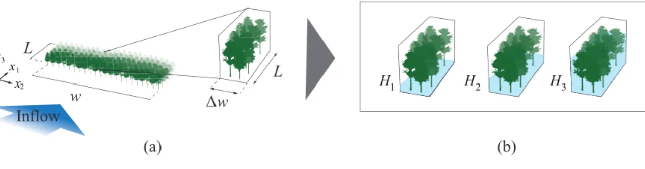
(i) We prepare a “local test domain” (LTD) that contains a sufficient number of trees in a coastal forest, as shown in Fig. 2.3(a);
(ii) With various flow conditions at the local level, as illustrated in Fig. 2.3(b), a series of micro-scale flow simulations are conducted in a rectangular open channel, where the LTD is equipped;
(iii) Based on each of the numerical test results, the macroscopic characteristics relevant to the overall resistance caused by the trees are evaluated from the volume-averaging operation over the LTD; see Fig. 2.3(c);
The volume-averaging processes will be performed over the LTD, which is regarded as a representative elementary volume (REV) within the framework of porous media theory (Bear [2013]). In the following subsection, the LTD setup process is explained in detail.
2.3.2
Local test domain
The first step of the procedure is to set up the LTD from the whole structure of a coastal forest that contains a sufficient number of trees to be representative of the homogeneous feature. The extracted LTD is a spatially reduced subdomain of the
Inflow 2 x 3 x 1 x L L w Δw (a) (b) H 1 H2 H3
Figure 2.3: Concept of the 3D numerical flow tests (a) The LTD established as a spatially reduced domain of the overall forest (b) Numerical simulations conducted with various inflow depths ˆh=h1, h2,... as well as the inflow velocity ˆu1
overall forests. And this LTD is equipped in a rectangular channel, as shown in Fig. 2.3(a). This subdomain is used for the 3D simulations to numerically ‘measure’ the trees’ resistance to flow in the next step.
In previous studies with purposes similar to ours, the streamwise length of the LTD is reduced to accommodate only a few trees. For example, Wang et al. [2015] employed a periodic LTD, called a unit cell, in which cylinders are vertically located to develop a surface water model. Lee and Yang [1997] also investigated flows in a 2D unit cell with emerged cylinders. However, Maza et al. [2015] reported that only the length of a forest is relevant to the overall wave damping. From referring to the knowledge mentioned above, we set the streamwise length of the LTD is equal to L. Meanwhile, the width of the LTD, ∆w, can be set to be considerably smaller than the width of the overall forest, w, to contain only a few trees since the transverse direction has little effect on damping. Maza et al. [2015] also reported that the distribution of trees, which is quite random in a native forest, is not as influential as the density. Therefore, trees are assumed to be homogeneously arrayed in the LTD to have an equivalent population per unit area to the original forest. Specifically, the arrangement can be periodic, as often assumed in various approaches for multiscale modeling.
Our numerical flow tests for the LTD are established by referring to the hydraulic experiments conducted by Hayashi et al. [2015], in which miniature trees located in an open channel. A portion of the actual miniature forest employed by Hayashi et al.
[2015] is illustrated in Fig. 2.4(a), in which the staggered arrangement of miniature trees that locates in the central part of the open channel. The domain surrounded by the red-colored solid line shown in Fig. 2.4(a) defines the LTD for the numerical flow tests.
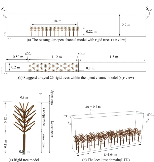
Fig. 2.5 shows the LTD, which is equivalent to the rectangular open channel domain, containing rigid trees that is used for micro flow simulation. As described in Fig. 2.5(a), (b), the length, the width and height of the channel are L = 2.112(m),
w = 0.2(m) and H = 0.5(m), respectively. An array of 26 trees is implemented with
a staggered arrangement, as illustrated in Fig. 2.5(b), and the shape of a rigid tree is illustrated in detail in Fig. 2.5(c). The rigid tree models are generated by referring to the hydraulic experiments performed by Hayashi et al. [2015].
2.3.3
Condition for numerical flow tests
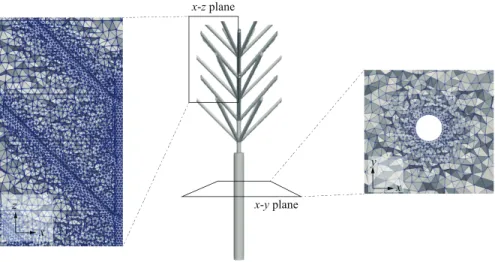
With the help of stabilized finite element method (Tezduyar [1991], Brooks and Hughes [1982]) and phase field method (Chiu and Lin [2011], Takada et al. [2013]), 3D Navier-Stokes equation (2.5) is solved for numerical flow tests. Precise explanations of these numerical schemes are presented in appendix A. FE mesh discretization by the tetrahedron 4-node elements is illustrated in Fig. 2.6 with the size of representative meshes summarized in Table 2.1.
The non-slip boundary conditions are imposed on the surfaces of trees and bottom (2.7), and also both side surfaces are periodically connected (2.9). On the upwind surface of the rectangular channel, the following inflow condition ˆu is applied on the
surfaces perpendicular to the overall flow direction, i.e., the x1-direction:
u|S in = ˆu = ˆ u1 0 0 , (2.10)
where ˆ• indicates prescribed values. A nonreflecting boundary condition is given to the outflow surface Sout. So that the flow in the LTD is composed of water and air, the two-phase flow simulation is realized. Thus, the inflow depth ˆh, which is the
vertical position of the interface, is prescribed to determine the flow rate of water in the inflow condition as described in Fig. 2.3.
It should be noted that the inflow conditions for numerical flow tests in the LTD are not necessarily the same as those in the open channel. As explained previously, since the numerical flow tests are carried out in the entire domain of the open channel, two inflow parameters, ˆu and ˆh, are applied to the boundary surface of the channel S. However, only flow inside the LTD domain Y is utilized in the numerical flow test
evaluation process. Considering that, we shall define the ⟨•⟩ as an evaluation index for numerical flow tests as:
⟨•⟩ = |Y1
f|
∫
Yf
• dV, (2.11)
where |Yf| means the volume of fluid in the LTD. The value ⟨•⟩ in (2.11) represents the volume averaged value over the LTD.
Also, the following time averaging operation will be applied to some time varia-tional value: ¯ • = 1 T ∫ t+T t • dt. (2.12)
Here, we take a general definition of averaging time scale proposed in the research of large-scale flow field by Gyr and Rys [2013] as follows:
T ≈ L
ˆ
u1
, (2.13)
where ˆu means inflow velocity and L indicates the length of the open channel.
Table 2.1: Information of the open channel model that consists of the rigid trees models that consists of the local test domain (LTD)
Total number of FE nodes 6,177,902
Total number of FE meshes 35,313,776
Size of representative meshes 2.0e-2 Size of meshes around tree models 1.0e-3
w = 0.8 m l = 0.1 m x 1 x 2
Figure 2.4: (a) The staggered arrangement of 97 miniature trees in the open channel used in the laboratory experiments by Hayashi et al. [2015]
2.4
Validation analysis
In order to confirm the validity of the established LTD, and the reliability of numerical flow tests, we conduct several 3D numerical flow simulations as case studies.
The similar LTD that consists of the array of the same sized-cylinders is examined as the comparative study to investigate the effects of trees morphology on the flow attenuation evaluation.
Discussion for the validity of the numerical flow tests are provided by comparison with the experimental results by Hayashi et al. [2015]. Note that more plain verifi-cation for the 3D direct numerical simulations with stabilized FEM and Phase-Field method is also provided in A.3.
2.4.1
LTD with rigid trees models
Table 2.2 shows the inflow conditions and corresponding case names for the numerical simulations. These inflow conditions are set up by referring to the hydraulic experi-mental results conducted in the open channel described in Fig. 2.4(a)(Hayashi et al. [2015]).
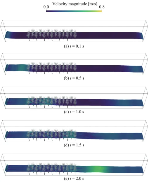
A resultant flow in Case-A is visualized in Fig. 2.7. The array of woods is colored white, and the velocity distribution of the surface flow at each time step is provided. After the flow passes through the trees at t = 2.0 s, the wake behind each tree can
be observed, as shown in Fig. 2.7(c). The flow speed increases locally in the spaces between downstream trees, as demonstrated in Fig. 2.7(d). These visualized flow convinced us that the patchy flow through rigid trees is successfully simulated by the stabilized finite element scheme and Phase-Field method. We can also recognize that the flow speed is attenuated behind the branches on the upstream side. These observations indicate that the complex shape of branches can constitute a severe factor influencing the evaluation of flow attenuation.
Table 2.2: Inflow conditions of 3D direct numerical simulations on the LTD consists of 26 rigid trees/cylinders. A set of initial flow speed ˆu1 and depth ˆh
Case Inflow velocity ˆu1(m/s) Inflow depth h (m)
A 0.30 0.10
B 0.50 0.25
C 0.30 0.33
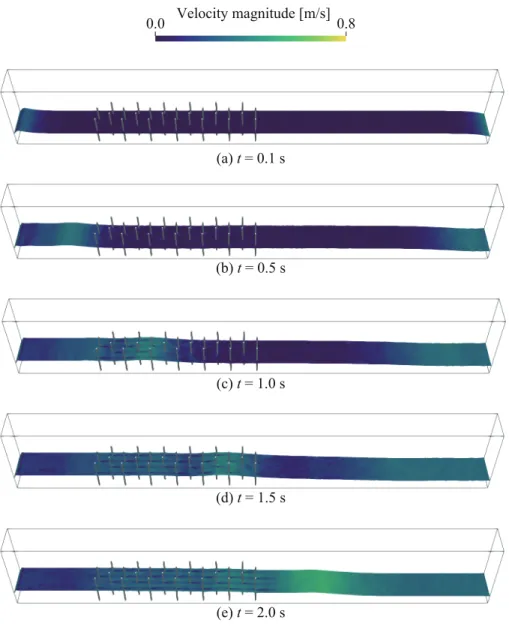
For the further evaluation on the effects of branches, we conduct the comparative simulations with the array of simple cylinders, which are the obstacles without any branches. Fig. 2.8 shows the open channel consists of the 26 cylinders. All size of the open channel are identical to the equipment provided in Fig. 2.5. The diameter and the height of each cylinder is same to those of the rigid tree model illustrated in Fig. 2.5(d). The result of the numerical simulations that are carried out with the inflow conditions Case A (Table 2.2) are provided in Fig. 2.8. As well as the observations to the flow through the rigid tree models in Fig. 2.7, the flow speed is also increased in the space between the cylinders. However, we can found the possibility of the decreased attenuation from the wake tendency. While the number of the wake behind the cylinders around t = 2.0 (s) is same to the number of the cylinders, the number of wake behind trees is increased than the number of the trees because the branches are exposed to be the water surfaces.
To quantitatively evaluate the difference between the resistance effects of rigid trees and that of cylinders, following indices are calculated in both type of simulations:
Depth reduction rate = ∆h
hin
× 100 = hout− hin
hin
× 100 (%), (2.14)
Non-hydrostatic pressure loss = 1
|∂Y+| ∫ ∂Y+1 p dΩ− 1 |∂Y−1| ∫ ∂Y−1 p dΩ (Pa). (2.15)
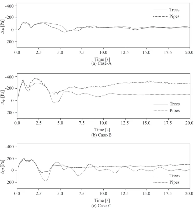
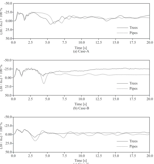
The time variations of depth reduction rate and the pressure loss in all cases are pre-sented in Fig. 2.10, Fig. 2.11. Comparing the solid lines and dashed lines described in Fig. 2.10(a) shows that both rigid trees and cylinders may have comparable resistance effects in Case A. This is because the rigid trees can be essentially the same as the cylinders under the stem-submerged depth level as anticipated. A similar tendency is also can be seen in the comparison between the depth reduction rate of two models in Case A in Fig. 2.11(a). Differently, the temporal values measured in Case B provided in Fig. 2.10(b) shows the distinct difference between the attenuation effects of trees models and that of cylinder models. We can also understand that the trees models have relatively large depth reduction effects compared to the pipes from the temporal data presented in Fig. 2.11(b). Considering that Case B is carried out with a canopy submerged-depth level, these enhanced flow attenuation effects in trees models are caused by the existence of branches. Consistent with the above-mentioned insights, flow attenuation-effects of trees model are also larger than that of cylinders in Case C by referring to the Fig. 2.10(c), Fig. 2.11(c).
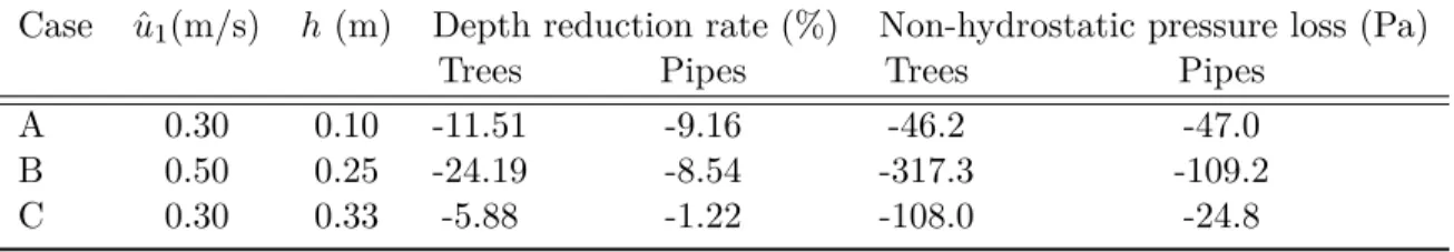
Using both (2.12) and (2.13) give the time averaged values of the depth reduction rate and the non-hydrostatic pressure loss as summarized in Table 2.3. Regardless of the kind of obstacles established in the LTD, the values of the stem-submerged depth case (Case A) are almost identical. On the other hand, the values of the canopy submerged-depth cases (Case B, C) shows the significant difference between the cylinder models and the rigid tree models. Both depth reduction rate and pressure loss caused by the rigid tree models are three times bigger than those caused by the cylinders These results reasonably agree with the observations to the data plotted in Fig. 2.10, Fig. 2.11 and strongly confirm the increased flow attenuation arise from the complex shape of tree models. As mentioned in the previous chapter (Chapter
1), a lot of early studies simulated the flow through the coastal vegetation with the cylinder obstacles (e.g., Maza et al. [2015]). However, as we uncovered, the effects of trees-like structures on the flow are different from that of the cylinders if they have branches, canopies. Especially, the resistance of mangrove trees, which are famous for their mitigation performance against past huge tsunamis (Kathiresan and Rajendran [2005b]), might be underestimated in the previous numerical simulations because their complex root systems are exposed to be the water flows. On the whole, we can convince that the established rigid trees in the LTD is worth to investigate by numerical flow tests.
Table 2.3: Comparison between the direct numerical simulations on the rigid trees and that on the cylinders. A set of initial flow speed ˆu1 and depth ˆh, and the observed
values of the depth reduction rate (2.14) and the loss of non-hydrostatic pressure (2.15).
Case uˆ1(m/s) h (m) Depth reduction rate (%) Non-hydrostatic pressure loss (Pa)
Trees Pipes Trees Pipes
A 0.30 0.10 -11.51 -9.16 -46.2 -47.0
B 0.50 0.25 -24.19 -8.54 -317.3 -109.2
C 0.30 0.33 -5.88 -1.22 -108.0 -24.8
2.4.2
3D numerical flow simulations
Now, we examine the reliability of the 3D flow simulations from the comparison with the hydraulic experimental results. Fig. 2.12 shows the streamwise velocity distribution in vertical direction obtained from several case study simulations (Table 2.2) on the rigid trees and the cylinders. The circle plots indicate the hydraulic experimental data by Hayashi et al. [2015]. The data obtained at the inflow surfaces Fig. 2.12(a)(c)(d) shows that the established boundary conditions (2.7), (2.10) cause the minor difference from the experimental results. Although the blue plots near the bottom surface (z=0.0) in Fig. 2.12(a)(c)(d) are smoothly transitioned to u=0.0 in line with the well-known hydraulic laws, the solid lines dramatically change near the
bottom surface. We reasoned that discontinuity between the non-slip boundary (2.7) and the inflow conditions (2.10) would affects this conflict. It should, however, be noted that this difference is unpleasant but is not a serious problem for the reliability of the numerical flow tests. The solid lines provided in Fig. 2.12(d)(e) indicates that our simulations can excellently reproduce the disturbance of the flow through the rigid tree models.
Fig. 2.13 shows the surface location of water flow obtained from the direct nu-merical simulations on the rigid tree models. The surface location of the simulated water flow (solid lines) is in the upper zone compared to that of the experimental flow (dots). Our simulations on the rigid trees seem to underestimate the flow-depth attenuation effects especially in canopy submerged depth cases (Case B, C in Fig. 2.13(b)(c)). However, such underestimation tendencies of rigid tree models would be acceptable because the experimental data was obtained with the plastic-deformable branches. We also convinced that the fewer branches in rigid trees also contributed to the gap from the plastic trees in which a large number of branches were mounted. Considering that the cylinder models have no branch, more severe underestimations of the dashed lines mean that the larger number of the branches may lead the solid lines-location to the dots plots locations.
The comparison between the solid lines and the dashed lines in Fig. 2.12 also provides several insights for the reliability of the simulations with trees-canopy mod-eling. The rigid tree models are superior to the cylinders in the reproduction of the velocity disturbance (Fig. 2.12(c)(d)) and the water surface. Notably, the streamwise velocities behind the canopy (0.1≤ z ≤ 0.22) are largely decreased compared to that behind the cylinders.
We can conclude that our numerical simulations have enough ability to simulate the flow through the complex shaped-structures, such as rigid trees models and to be employed as the numerical flow tests in multiscale modeling.
2.5
Summary
In this chapter, we proposed multiscale modeling for flow through trees. We first separated the flow into two spatial scales: micro-scale, and macros-scale. Each scale flow was defined as a 3D flow described by the Navier-Stokes equation and 2D flow described by the shallow water equation. And then, the procedure of numerical flow tests, which is a three-dimensional simulation of micro-scale flow, has been provided. According to the proposed procedure, we set up the open channel domain that consists of a sufficient number of rigid trees as the LTD. With this LTD, numerical flow tests are to conducted with various inflow conditions. From results obtained from a series of numerical flow tests, macroscopic characteristics for 2D shallow water simulation are meant to be obtained. In order to confirm the reliability of established LTD and the capability of numerical simulations, we conducted several case study-simulations on the array or rigid trees, as well as the array of the same sized cylinders. Comparison of the flows through those two structures demonstrated the serious effects of canopy-shape and such a detailed tree modeling is worth to do. and the advantage of rigid trees models for the simulations of the previous hydraulic experiments. The profile of the flow depth/velocity of the 3D simulations on rigid trees models reasonably agree with that obtained from the experimental flow through the plastic-deformable trees although there are minor difference of trees modeling or inflow conditions.
In the following two chapters, several evaluation methods for converting micro-scale flow characteristics into the expression of the tree’s presence in macro-micro-scale flow are examined in detail, along with the underlying theories.
(b) Staggerd arrayed 26 rigid trees within the opent channel model (x-y view) (a) The rectangular open channel model with rigid trees (x-z view)
(c) Rigid tree model
0.5 m 0.22 m 1.04 m 0.2 m 1.12 m 0.1 m 0.8 m 0.01 m 0.50 m 1.5 m in S Sout x y x z L=1.04 m Δw = 0.2 m
(d) The local test domain(LTD)
T runk z one Ca nopy z one U ppe r z one L ow er z one 0.1 m 0.12 m
Figure 2.5: (a)Test domain for 3D numerical flow simulation. It consists of 26 trees. (b)The staggered arrangement of 26 miniature trees in the open channel. (c)Miniature tree models (d) The local test domain (LTD) used for a series of numerical flow tests
x y x-y plane x-z plane x z
Figure 2.6: FE mesh information
Velocity magnitude [m/s] 0.0 0.8 (a) t = 0.1 s (b) t = 0.5 s (c) t = 1.0 s (d) t = 1.5 s (e) t = 2.0 s
Figure 2.7: Results of direct numerical simulations on 26 rigid trees inside the open channel
(b) Staggerd arrayed 26 rigid trees within the opent channel model (x-y view) (a) The rectangular open channel model with rigid trees (x-z view)
(c) Rigid tree model
0.5 m 0.22 m 1.04 m 0.2 m 1.12 m 0.1 m 0.01 m 0.50 m 1.5 m in S Sout x y x z L=1.04 m Δw = 0.2 m
(d) The local test domain(LTD)
0.22 m
Figure 2.8: (a) Open channel domain that consists of 26 cylinders. (b)The stag-gered arrangement of cylinders. (c) Cylinder model (d) The local test domain (LTD) containing the cylinders
Velocity magnitude [m/s] 0.0 0.8 (a) t = 0.1 s (b) t = 0.5 s (c) t = 1.0 s (d) t = 1.5 s (e) t = 2.0 s
Figure 2.9: Results of direct numerical simulations on 26 rigid pipes inside the open channel
0.0 2.5 5.0 7.5 10.0 12.5 15.0 17.5 20.0 Time [s] Trees Pipes -400 0 -200 200 0.0 2.5 5.0 7.5 10.0 12.5 15.0 17.5 20.0 Time [s] Trees Pipes -400 0 -200 200 0.0 2.5 5.0 7.5 10.0 12.5 15.0 17.5 20.0 Time [s] Trees Pipes -400 0 -200 200 [P a] (a) Case-A (c) Case-C (b) Case-B [P a] [P a]
Figure 2.10: Temporal variation of non-hydrostatic pressure loss (2.15) observed in Case A, B, C.
0.0 2.5 5.0 7.5 10.0 12.5 15.0 17.5 20.0 Time [s] -50.0 0.00 -25.0 25.0 50.0 Trees Pipes Time [s] 0.0 2.5 5.0 7.5 10.0 12.5 15.0 17.5 20.0 -50.0 0.00 -25.0 25.0 50.0 Trees Pipes Time [s] 0.0 2.5 5.0 7.5 10.0 12.5 15.0 17.5 20.0 -50.0 0.00 -25.0 25.0 50.0 Trees Pipes ( Δ h / h in ) × 100 % (a) Case-A (c) Case-C (b) Case-B ( Δ h / h in ) × 100 % ( Δ h / h in ) × 100 %
Figure 2.11: Temporal variation of depth reduction rate (2.14) observed in Case A, B, C.
0.3 0.2 0.1 0.0 0.0 0.2 0.4 0.6 0.0 0.5 1.0 0.11 0.04 0.3 0.2 0.1 0.0 Trees Pipes 0.14 0.04 Trees Pipes 0.3 0.2 0.1 0.0 0.0 0.2 0.4 0.6 0.0 0.5 1.0 0.3 0.2 0.1 0.0 0.18 0.12 Trees Pipes 0.18 0.12 Trees Pipes 0.3 0.2 0.1 0.0 0.0 0.2 0.4 0.6 0.0 0.5 1.0 0.3 0.2 0.1 0.0 0.15 0.10 Trees Pipes 0.15 0.10 Trees Pipes u [m/s] u [m/s] u [m/s] u [m/s] u [m/s] u [m/s] z [m] z [m] z [m] z [m] z [m] z [m]
(a) Case-A: Inflow (b) Case-A: Outflow
(c) Case-B: Inflow (d) Case-B: Outflow
(e) Case-C: Inflow (f) Case-C: Outflow
Figure 2.12: Velocity distribution in vertical direction
Comparison between 3D direct simulations on rigid trees and hydraulic experiments on plastic trees-model
(a) Case-A 0.3 0.2 0.1 0.0 0.4 0.5 0.0 0.5 1.0 1.5 -0.5 D ept h h [m ] Trees Pipes Hayashi et al.2015 x [m] (c) Case-C 0.3 0.2 0.1 0.0 0.4 0.5 0.0 0.5 1.0 1.5 -0.5 D ept h h [ m ] x [m] (b) Case-B 0.3 0.2 0.1 0.0 0.4 0.5 0.0 0.5 1.0 1.5 -0.5 D ept h h [m ] x [m] Trees Pipes Hayashi et al.2015 Trees Pipes Hayashi et al.2015
Figure 2.13: Depth of flow through the rigid trees/cylinders(3D direct numerical simulations) and plastic trees (hydraulic experiments by Hayashi et al. Hayashi et al. [2015]) in streamwise direction x
Energy balance-based multiscale
evaluation
3.1
Introduction
Based on the procedure presented in the previous chapter, we conduct numerical flow test for evaluating the resistance of trees in macro-scale flow from energy balance re-lation with micro-scale flow. We first assume the work rate done by the force term in macro-scale flow can be evaluated from the energy dissipation caused by the micro-scale flow stress. With this assumption, we set up an energy balance relationship between micro-scale and macro-scale from the operation to both momentum equa-tions. To evaluate the energy balance between micro-scale flow and macro-scale flow, we carry out a series of numerical flow tests for the LTD in accordance with Chapter 2. The values of energy dissipation, which assumed to include the effects of trees’ presence, are calculated from several numerical flow tests with several inflow condi-tions. We examine the evaluated energy dissipation values through the comparison with predicted values of work rates of macroscopic stress term based on a classical formulation. And then, energy values are converted to the roughness parameter for the macro-scale flow simulations. Some vilification analyses by the 2D shallow wa-ter flow simulations are provided to investigate the validity of obtained roughness parameters and presented an energy balance assumption.
3.2
Mechanical energy balance between two scales
3.2.1
Energy dissipation in 3D micro-scale flow domain
In the LTD, the motion of flow is described by the 3D Navier-Stokes momentum equation Eq. (2.5), as is explained in Sec. 2.2.2. After performing multiplication with the velocity vector u = [u1, u2, u3] and integrating over the domain Yf, the momentum equation Eq. (2.5) is rewritten as the mechanical energy balance equation inside the LTD (Mei et al. [1989]):
∫ Yf ρDui Dt ui dV =− ∫ Yf ρgδi3ui dV + ∫ ∂Yf {−P δij + τij}njui dS− 1 2µ ∫ Yf τijτij dV, (3.1) where ni denotes the unit normal vector orthogonal to the boundary surface ∂Y of
Yf.
Each integral in the right-hand side of Eq. (3.1) indicates the rate of work done by body force, that the rate of work performed on the boundary surface ∂Yf (2.8) and the viscous dissipation rate inside the volume Yf, respectively. Here, we define the sum of the second term and third term as the total energy rate caused by the fluid force σ· n inside the domain as:
E = ∫ ∂Yf {−P δij + τij}njui dS− 1 2µ ∫ Yf τijτij dV. (3.2)
Hereinafter, scalar value defined in Eq. (3.2) is called as as microscopic flow dissipa-tion.
3.2.2
Rate of work done by 2D macro-scale flow stress
Similar to the operation we did for 3D Navier-Stoke momentum equation in previous section3.2.1, the equation that states balance of energy rate in 2D shallow water flow can be obtained by taking the scalar products of the momentum equation Eq. (2.1)
![Table 3.2: Results of numerical flow tests for rigid trees in the LTD A set of time averaged mean depth [h], mean velocity ⟨ u ⟩ by Eq](https://thumb-ap.123doks.com/thumbv2/123deta/5897920.1048997/58.918.262.710.254.550/table-results-numerical-tests-rigid-trees-averaged-velocity.webp)
![Figure 3.1: Temporal variation of the mean velocity |⟨ u ⟩| (m/s) and the mean depth [h] (m) at each case](https://thumb-ap.123doks.com/thumbv2/123deta/5897920.1048997/66.918.172.802.208.962/figure-temporal-variation-mean-velocity-mean-depth-case.webp)
