160
Complex
Rheology in
a
Simple Lattice
Gas
Model
Akinori Awazu
Department ofPhysics, University of Tokyo,
Hongou7-3-1,Bunkyou-ku, Tokyo 113-0033, Japan.
1
Introduction
$\mathrm{t}\backslash ^{\tau}\prime \mathrm{e}$
, investigatethe transport behaviors of
a
simplelattice gassystemwith aperiodic boundary,which consists of only two particles interacting repulsively and the potential forces acting
on
the1n. Nonequiiibriumlattice gases
are
sim plemathem aticalmodels, which havebeen useful andimportant instudies of the several properties ofnonequiiibrium system $\mathrm{s}$with
numerous
degreesoffreedom [1]. Under nonequiiibrium co1ldition$\mathrm{n}\mathrm{s}$, lattice
gas
systems have been known to showsome nontrivial phenomena, such as the
appearance
of long-range spatial correlations[3] and anomalous drift motions[2], even if the syste$\ln$ involves only two particles. Inour
system, thefollowing novel transport properties
are
found when onlyone
particle is driven by an externaldriving field; With the increase in the mean velocity of the driven particle, the coefficient of
effective drag of this particle ($=$
jdriving
field strength]/[mean velocity]) varies in the form,increase $arrow$ decrease$arrow$ increase $arrow$decrease. Moreover, under otherconditions, thecoefficient of
effectivedragshows change similar to that observed in the shear-thickening polymer
or
colloidalsolutions.
2
Model
Now,
we
introducea lattice gasmodel,which is thesameas
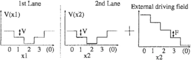
thatstudiedinourprevious paper[2].We consider a lattice systemwith two parallel one-dim ensional lanes where each lane involves
$L$ sites with
a
periodic boundary. Each lane contains onlyone
particle which moves randomlyto the nearest sites withoutchanging lanes. The sites occupied by particles in the 1st and 2nd
lanes
are
denoted $x_{1}$ and $x2$, respectively, whichare
givenas
integer$\mathrm{n}$ mbers from0
to $L-1$.
Theeffect ofpotentialforcesactingon theparticles is described by the followingHamiltonian:
$H(x_{1}, x_{2})=\mathrm{V}(\mathrm{x}))$$+V(x_{2})+V_{12}(x_{1}, x_{2})$, (1)
where $V(x)$ represents the one-body potential
on
each lane, and $V_{12}(x_{1\}}x_{2})$ represents thein-teraction potentialbetween the two particles. Furthermore,
an
external driving field is appliedto theparticle
on
the 2nd lane. Wedenote the fieldstrength $F$.
181
Figure 1. Illustrations of effects of potential and external field ineachlane.
The time evolution of this systemis described by the iteration of the following three steps.
First,
one
ofthe two particles is randomly chosen. Let the position of the chosen particle be$x$.Second, its neighboring site $y$, $x$ –1 or$x+1$, is randomly chosen. Third, the chosenparticle
moves
from$x$to $y$with thefollowing probability$c(x, y;x_{1}, x_{2})= \frac{1}{1+\exp[Q(xarrow yjX_{1},X_{2})/k_{B}^{\wedge}T]}$, (2)
with
$Q(xarrow y;x_{1}, x_{2})=H(x_{1}’, x_{2}’)-H(x_{1}, x_{2})-F(x_{2}’-x_{2})$, (3)
where $(x_{1}’, x_{2}’)=(x_{1}, y)$when$x=x_{2}$, and $(x_{1}’, x_{2}’)=(y, x_{2})$ when$x=x_{1}$
.
$T$is temperature andthe Boltzmann
constant
$k_{B}^{n}$ is set 1. Here,thetime stepisgiven by [No. of aboveiterations] / [No.of particles $(=2)]$
.
Specifically, we study the
case
where $V(x)$ $=V|L/2-x|$ (Fig. 1), and $V_{12}(x_{1}, x_{2})=I\delta_{x_{1},x_{2}}$using the $L\cross$ $L$ unit matrix $\delta_{ij}$. Also,
we
focuson
thecase
$L=4$. We found that this size isthe minimum required to exhibit the phenomenon
we
demonstrate in the presented paper.3
Simulation
Now,
we
demonstrate a simulation of this system. In particular,we
focus on thecases
with$F$
as $|F|<I+V$
and $T$ is small enough compared to I and $V$.
Then, the influences of thepotentialforces andthe interactions
are
strong compared to those of thedriving field. Iri orderto characterize the system, we define the
mean
velocity of the driven particle (inthe 2nd lane)in steady state $u$
as
the difference of the long time average of the moving ratio in the positiveand negative directions. Here, the direction$x_{i}$ :0 $\neg 1\neg$ $.,$
.
$arrow(L-1)arrow 0arrow$is positive. Forsim plicity, $I=1$ and $F>0$ are set.
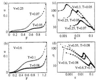
Figures $2(\mathrm{a})$ and (b) show $u$ as a functionof$F$ for (a) $V=0.25$with $T=0.05$ or $T=0.07$
and (b) $V=0.6$ with$T=0.0\mathrm{S}$
or
$T=0.1$. As shown in them, two typesof $F-u$ relations,i) $u$ increases steeply with $F$, $\mathrm{i}\mathrm{i}$)
$u$ increases slowly with $F$, appear depending
on
the range182
(a) $\mathrm{V}=025$ ‘ $\mathrm{u}$ $\mathrm{T}=007$ $.\star$ 01 $.*\cdot\mu^{l}$.
$*^{\mu\cdot\star\mu\cdot\wedge}\cdot/^{*\mathrm{T}=005}’ k$ $0_{0}$ 02 04 06 08 I $\mathrm{F}$ (b).
(d) $\mathrm{V}=0$$6$.
100 $01\mathrm{u}$ $\mathrm{T}=01$ $* \int$ $\eta$ $\vee=($ $P’..*\cdot.\mathrm{T}l=0^{\cdot}08’.d\cdot\#^{m^{\vee’}}*\cdot$ 10.
$\backslash \mathrm{V}_{\backslash }=,055$, $\mathrm{T}=008$ $.-\sim.\sim_{1}.$ , , 06,$\mathrm{T}=008$ $\mathrm{V}=06,\mathrm{T}=01$ $0_{0}02$ $04$ $06$ $08$ $1$ 0001 001 01 $\mathrm{F}$ $\mathrm{u}$Figure 2: $.\backslash \mathrm{I}\mathrm{e}\mathrm{a}\mathrm{n}$ velocity
$u$ as
a
function of $F$ for (a) $V=0.25$ with $T=0.05$ or$T=0.07$ and(b) $V$ $=0.6$ with $T=0.08$ or $T=0.1$, and coefficient of effective drag $\eta$ as
a
function of$u$ for(c) $V=0.25$
or
$V=0.3$ with $T=0.05$ or$T=007$ and (d) $V=0.55$ or $V=0.6$with T—0.08or$T=0.1$.
driven particle $\eta$ defined as $F/u$
are
straightforwardly obtained. Figures$2(\mathrm{c})$ and (d) show
$\eta$
as
a function of $u$ for (c) $V=0.25$or
$V=0.3$ with $T=0.05$ or $T=0.07$ and (d) $V=0.05$or $V=0.6$ with $T=0.08$ or$T=0.1$. As shown in Fig $2(\mathrm{c})\eta$ varies inthe form, increase $arrow$
decrease $arrow$ increase $arrow$ decrease, withthe increase in$u$ in the
case
with$V<I/2$ anda
small $T$(for example $V=0.3$ and $T=0.05$).
When the smaller $V$ and a little larger $T$
are
given (for example, $V=025$ and $T=\zeta$)$.07)$,thechange in $\eta$ becom es less sharp, and simpler in the form, increasing$arrow$ decreasing, with the
increasein $u$ (Fig. $2(\mathrm{c})$). In this case, the u- $\eta$ profile is given in
a
form qualitatively similarto that between the shear rate and shear viscosity coefhcient of the shear-thickening polymer solutionsobtained experimentally$[4, 5]$
On
the otherhand, ifa
larger$V$isgivenas
inthe range$I/2<V<I$
(forexam $\mathrm{p}\mathrm{l}\mathrm{e}$, $V=0.55$ and $V=0.6$),$\eta$ varies in thefo
$\mathrm{r}\mathrm{r}\mathrm{n}$, decrease $arrow$ increase $arrow$
decrease, with the increase in $u$ independently of$T$ (Fig. 2(d)). In this case, the $u-\eta$ profile
appears qualitativelysimilartothat between the shear rate and shear viscositycoefficient ofthe
shear-thickeningcolloidal solutions obtained experim entally[6|.
4
Summary and discussions
In this paper,
we
investigated the transport behaviors of a simple nonequilibrium latticegas
system.
Our
resultscan be easily explained by theconsiderations of the transitionprobabilities183
uncover
the possible mechanism for several rheoiogical characteristics ofseveral soft materials.Detailed studies for the presented system $\mathrm{s}$ should be reported in the other paper in future[7].
Moreover, studies of extendedmodels, including
more
lanes or particles in thespace with moresites
or
continuousspace,
and the relations between such toy systems and either real systemsor more
realistic models of the polymerorcolloidal solutions[4, 5, 6] represent important futureissues.
The author thanks to M. Sano, and M. Otsuki for useful discussions. This research
was
supported inpart by a Grant-in-Aid for
JSPS
Fellows (10039).References
[1] B. Schim ttmann and R. K. P. Zia, Statistical Mechanics of DrivenDiffusive Systems
(Aca-demic Press, London, 1995).
[2] A. Awazu, J. Phys. Soc. Jpn. 74 (2005) 3127.
[3] H. Tasaki, cond-mat/0407262
[4] K. C Tarn,R. D. Jenkins, M. A. WinnikandD. R. Bassett, Macromolecules 31 (1998) 4149.
[5] S X. Ma and S L. Cooper, Macromolecules 34 (2001) 3294.
[6\rfloor E. Bertrand, J. Bibetteand V. Schmitt, Phys. Rev. E66 (2003)