Quantization Methods in Filtering and Applications to Partially Observed Stochastic Volatility Models(The 7th Workshop on Stochastic Numerics)

Quantization

Methods

in

Filtering

and

Applications

to

Partially

Observed Stochastic

Volatility

Models

Huyen

PHAM

Laboratoire de Probabiliteset ModelesAl\’eatoires CNRS, UMR 7599 Universite Paris 7 e-mail: [email protected] and CREST

October

12,

2005

Abstract

We presentsomerecentdevelopmentsonoptimalquantizationmethods for

discrete-time nonlinear filtering, Weanalyse first the quantization algorithm for the filter given

a fixed observation, and then the quantization of the filter process. This last study

is motivated by dynamic optimization problems under partial information arising for

example in finance in the pricing of American options under partiallyobserved

stochas-tic volatility models. Several numerical illustrations are carried out, emphasizing the

convergenceand the stability of the approximatefilter.

Key words :Nonlinearfiltering, Markovchain, quantization, stochastic gradient descent,

optimal stopping.

80

1

Introduction

Optimal quantization of randomvectors consists in finding the best approximationin $L^{p}-$

norm

of

a

random vector by

a

discrete random vector taking at most $N$ values. This

was

originally developed in the 50’s in the context of information theorywhere the basic

motivationwas to transmit efficiently

a

continuous stationary signal by

means

of

a

finite

number ofcodes (or quantizers)

.

More recently,thequantization approach

was

applied to

variousfields, andnotablyto numerical probability, whereit appears

as an

efficient spatial

discretization method forsolving multi-dimensionalproblems arisingtypically in finance.

In this article, wepresentrecentdevelopments of optimal quantizationmethodsapplied

to thenonlinearfiltering problem. Thisisform allythe situation where

we

facea stochastic

system whose evolution is governed by

a

hidden process that we observe only through

some

noise. Filtering is a traditional problem in probability and statistics, and

occurs

in

particular in a financial context where we can observe stock price but not its volatility.

Mathematically, theproblem is to

recover

the optimal filter, i.e. the conditionallawofthe

hidden process (the signal) given the past observations. For instance, standard filtering

problems in finance

are

the estimation of the law of the volatility given the past price

observations, and then the pricing ofderivatives and portfolio optimization in a partially

observedstochasticvolatilitymodel. Except

some

very specific

cases

like theKalman-Bucy

model, thereisnoexplicitsolutionforthe filterandone has to resort on numerical methods.

The various approaches proposed in the literature (particle methods, grid methods) rely

basically on the principle of finding a finite-dimensinal representation of the filter. We

presentherethe quantization approach for filtering introduced in [7],whichis

a

grid method,

and where

one

searchs for grids that fit optimally accordingto$L^{2}$

-norm

to the distribution

of the sign al. In these numerical methods, the filter is approximated for

a

given fixed

set ofobservations. However, inmany applications arising in dynamic optimization under

partial observation,

one

need to approxim ate the filter process where randomness is due

to past observation process. We thenpresent

a

quantization approach ofthe filterprocess

introducedin [9] and give

a

numericalapplicationto theproblemofoptimalstopping under

partialobservation.

The paper is organized

as

follows.

Section 2 formulates and

recalls

some

preliminaries

on the filtering problem. In Section 3,

we

present the quantization method for

approxi-matingthe filtergiven a fixedxobservation. Section

4

illustrates theresults with numerical

experiments. In Section 5, we introduce the quantization approachfor the approximation

of the filter

process,

and

we

deal in the last Section 6 with a numerical application to the

optimal stopping problem in

a

partiallyobserved stochastic volatility model.

2

Filtering

problem

for

discrete observations

2.1

General

framework

We consider a discrete time, partially observable process $(X, Y)$ _where $X$ represents the

state or signal process that

may

not be observable, while $Y$ isthe observation,

The

signal

probability transition (Pk) (i.e. the transition from time $k-1$ to time $k$), andinitial law

$\mu$. The observation sequence (Yk) is valued in

$\mathbb{R}^{q}$, suchthat thepair $(Xk, Yk)$ is

a

Markov

chain onthe probabilityspace $(\Omega \mathrm{P})\}$ and

(H) Thelaw of$Y_{k}$conditional

on

(Xk-U$Yk-1,$$Xk$),$k\geq 1_{7}$denoted$qk$(Xk-U,$Y_{k-1},$$Xk,$$dy’$),

admits a bounded density (calledsometimes local likelihood function) :

$y’$ $\mapsto$ $g_{k}(X_{k-1}, Y_{k-1}, X_{k}, y’)$

.

For simplicity,

we assume

that $Y_{0}$ is

a

known deterministic constant equal to yo-

No-tice that the probability transition of the Markov chain $(Xk, Yk)_{k\in \mathrm{N}}$ is then given by

$Pk$ ,$dx’)gk(x, y_{2}x’, y’)dy’$ with initial law$\mu(dx)\delta_{y0}(dy)$.

We denoteby $(F_{k}^{Y})$ the filtration generated bythe observation process $(Y_{k})$ and by $\Pi_{k}$

the filter conditional law of$X_{k}$ given$\mathcal{F}_{k}^{Y}$

:

$\Pi_{k}(dx)$ $=$ $\mathrm{P}$$[Xk\in dx| F_{k}^{Y}]$ , $k\in \mathrm{N}$

.

A typical caseof signal-observation model isgivenby the following scheme :

$X_{k}$ $=$ $F_{k}(X_{k-1\mathrm{t}}\epsilon_{k})$,

$Y_{k}$ $=$ $G_{k}(X_{k-1}, Y_{k-1},X_{k}, \eta_{k})$,

for

some

measurable functions F&, $G_{k}$, andwhere (ek) and $(\eta k)$ are two white noises. For

example infinance, $(X_{k})_{k}$isthe unobservable return$\mathrm{a}\mathrm{n}\mathrm{d}/\mathrm{o}\mathrm{r}$volatility ofstockprice$S$while

$Y_{k}=$ In$S_{k}$ isthelogarithm oftheobserved priceprocess $Y_{k}$ $=$ $Y_{k-1}+b(X_{k-1})+\sigma(X_{k-1})\eta_{k}$,

andgk is explicit once thedensityofthe white noise $\eta k$ is specified.

2.2

Filter evolution

We denote by $\mathrm{A}l(E)$ the set of finite nonnegative

measures

on

$(E, \mathcal{E})$ and by $\mathcal{P}(E)$ the

subset of probability

measures on

$(E, \mathcal{E})$. Itis known that$\lambda 4(E)$ is

a

Polish

space

equipped

with the weak topology, hence

a

measurable space

endowed

with the Borel $\mathrm{c}\mathrm{r}$-field. From

Markov property and Bayes formula, the filter

process

$\mathrm{I}\mathrm{I}k$ valued in $\mathcal{P}(E)$ satisfies the

filteringforward equation :

$\Pi_{0}$ $=$ $\mu$,

$\Pi_{k}(dx’)$ $=$ $\frac{\Pi_{k-1}H_{k}(dx’)}{\Pi_{k-}{}_{1}H_{k}(E)}$ $.= \frac{\int_{B}\Pi_{k-1}(dx)H_{k}(X_{\}}dx’)}{\int_{B}\Pi_{k-1}H_{k}(dx’)}$ (2.1)

where $H_{k}$ istheprediction-updating transition kernel given by :

$H_{k}(x, dx’)$ $=$ _$gk$($x$, Xk ,$x’,$$Y_{k}$)$P_{k}(x, dx’)$.

Hence, thecalculation from$\Pi_{k-1}$to$\Pi_{k}$is doneintwo steps:

a

first step of prediction, which

82

correction andupdating,which

uses

the

a

posterioriinform ation given bytheobservation at

time$k$viathe locallikelihoodfunction g%. We denote the relation (2.1) (whichisnonlinear

due the norm alization) from $\Pi_{k-1}$ to $\Pi_{k}$ by :

$\Pi_{k}$ $=$ $\overline{G}_{k}(\Pi_{k-1}, Y_{k-1}, Y_{k})$

.

Given afixed setofobservations,the filtering problem consistsin solvingorsimulating

by approximation this filtering equation valued in the infinite dimensional space $\mathcal{P}(E)$

(whenthestatespace$E$is continuous). We distinguish essentially three typesof methods:

-Analytical methods where

one

tries tosolve analytically theforwardequation. This is

explicitly possiblewhen$X$and$Y$

are

Gaussian

processes

leadingto the well-knownKalman

filter,which is

a

finite-dimensionalfilter completelycharacterizedbyits

mean

and variance.

Someextensionsarederived withthe so-called extended Kalm an filter. Wealso citerecent

work in [3], which derives

an

explicit filter of infinite dimension.

-Monte-Carlo methods :this approach consists basically in approximating $\mathrm{I}\mathrm{I}k$ by a

sequence of empirical

measures

associated to $\overline{N}$ interacting particles at each time $k$ and

simulate according to the $\mathrm{p}\mathrm{r}\mathrm{e}\mathrm{d}\mathrm{i}\mathrm{c}\mathrm{t}\mathrm{i}\mathrm{o}\mathrm{n}/\mathrm{u}\mathrm{p}\mathrm{d}\mathrm{a}\mathrm{t}\mathrm{i}\mathrm{n}\mathrm{g}$ mechanism given by the transition kernel

$H_{k}$.

-Grid methods$\sim$

. _{this consistsin approxirnatingthetransition kernel}$H_{k}$bya transition

matrix $\hat{H}_{k}$, which leads in turn to an approximate forward equation valued in

a

finite

dimensional space

We developin thetwo next sectionsoptimal quantizationmethods that belongtogrid

methods. It isalso of interest to approximate not only the filter for a given set of

obser-vations, but

more

generallythe filter process viewed

as

a

random

measure

function of the

uncertainty of the observationprocess. This willbe developedinthetwolast sectionswhere

aquantization approach isintroduced forapproximatingthefilter processwithapplications

to partial observation problems.

3

Approximate filter by optimal

quantization

(Fixed

obser-vation)

3.1

Short background

on

optimal

vector

quantization

The basic ideaof (quadratic) quantizationis to replace an $\mathbb{R}^{d}$-valued random

vector $X\in$

$L^{2}(\mathrm{P}, \mathbb{R}^{d})$, with probabilitylaw$\mathrm{p}_{X}$, by

a

randomvector taking at most _$N$values in order

tominimizethe induced$L^{2}$-error. For this, consider agrid_{$x=\{x^{1}, . , . , x^{N}\}$} of

$N$pointsin

$\mathbb{R}^{d}$ (we shalloftenidentify such

a

grid with a

$N$-tuple in$\mathbb{R}^{d}$),

and its Voronoi tesselations, that is Borel partitions $C_{1}(x)$, ,.., $C_{N}(x)$ of$\mathbb{R}^{d}$

satisfying :

$C_{i}(x)$ $\subset$ $\{u\in \mathbb{R}^{d}$ :

$|u-x^{\iota}|= \min j=1,$

. $,N|u-x^{j}|\}$, $\mathrm{i}=1$,$\ldots$,$N$.

Then,

one

defines the $x$

-Voronoi

quantization of$X$

as

the closest neighbour projection of

$X$

on

thegrid $x$

:

$\hat{X}^{x}$

whose discrete probability law$\mathrm{P}_{\hat{X}}$ is characterized by :

$\hat{p}i|.=\mathrm{P}_{\hat{X}}(x^{i})=\mathrm{P}x$(Ci (x)), $\mathrm{i}=1$,

.. .

’$N$.

Inthe sequel, we often dropthe exponent $x$in $\hat{X}^{x}$ when there is

no

ambiguity, and

we

say

that$\hat{X}$

is

a

quantizer of$X$. The$L^{2}$-error inducedbythisprojection, called$L^{2}$-quantization

error, is $||X-\hat{X}||_{2}$

.

As

a function of the $N$-tuple (grid) $x=(x^{1}, \ldots x^{N})\}\in(\mathbb{R}^{d})^{N}$, the

squareofthe $L^{2}$-quantization error, calleddistorsion, iswritten as :

$D_{N}^{X}(x)=||X-\hat{X}||_{2}^{2}$ $=$ $\int\iota=1\mathrm{m},\acute{.}1..\mathrm{n},N|u-x^{\mathrm{i}}|^{2}\mathrm{P}_{X}$(du). (3.2)

First, notice bydefinitionof theclosestneighbourprojection thatthe$L^{2}$-quantization

error

is the minimum of$L^{2}$

error

_{$||X-Y||_{2}$} among all random variables $Y$ taking values in the

grid$x$. Then, twoquestionsarise naturally: forfixed $N$, isthere

an

optimal grid$x^{*}$ which

minimizes the $L^{2}$-quantization

error

(or equivalently the distorsion), and how does this

minim um behave when $N$goes toinfinity7 The latter question isansweredby the so-called

Zadortheorem :

Theorem 3.1 (see [4])

Assume that$X\in L^{2+\epsilon}(\mathrm{P}, \mathbb{R}^{d})$

for

some

$\epsilon$ $>0$ andset $f$ the Radon-Nykodim density

of

$\mathrm{P}_{X}$

in its decomposition with respect to the Lebesgue

measure

$\lambda_{d}$

on

$\mathbb{R}^{d}$

. Then,

$\lim_{N}N^{\frac{2}{d}}\min_{x}$ $||X-\hat{X}^{x}||_{2}^{2}$ $=$

$J_{d}||f||_{\phi+}$,

where $||f||_{r}=$ $(f |f|^{r}d\lambda d)^{1/r}$

for

$r>0$, and$J_{d}$ is aconstant depending on$d_{f}$ corresponding

to the

_uniform

distribution

on

$[0, 1]^{d}$.

Remark 3.1 In dimensions d $=1$ and2, $J_{1}= \frac{1}{12}$ aaand $\mathrm{J}_{2}=\frac{5}{18\sqrt{3}}$. forr d $\geq 3$, $J_{d} \sim\frac{d}{2\pi e}$

as

dgoes to infinity.

The optimal$N$-quantization problem thatconsistsindeterm ining

a

grid$x^{*}$, which

min-imizes the $L^{2}$-quantization error, relies

on

the property that the distorsion is continuously

diflerentiable atany$N$-tuplehaving pairwise distinct components, with

a

gradientobtained

by formal differentiation in (3.2)

:

$\nabla D_{N}^{X}(x)$ $=$

2

$( \int_{C,(x)}(x^{i}-u)Px(du))1\leq i\leq N$ (3.3)

A quantizer $\hat{X}=\hat{X}^{x}$ issaid stationaryif the associated $N$-tuple _$ satisfies

$\nabla D_{N}^{X}(x)$ $=$ 0.

Anoptimalquantizer is astationary quantizer. From (3.3),

we

have theuseful propertyof

stationary quantizers :

84

The integral representation (3.3) of $\nabla D_{N}^{X}$ suggests,

as

soon as independent copies of $X$

can be simulated, to implement a stochastic gradient algorithm (descent), in order to get

numerically a stationary quantizer. In our context, this leads to the Kohonen algorithm

or competitive learning vector quantization (CLVQ) algorithm, which also provides

as

a

byproduct

an

estimation of the weights $pi$ of the Voronoi tesselations associated to the

stationary quantizer. We refer to [8] for

a

description and discussion of the algorithm.

Optimal grids andtheircompanion parameters, i.e. weightsof theVoronoi tesselationand

distorsion, for thenormal distribution

are

available and downloadable

on

thewebpages of

Gilles Pages

or

Jacques Printems.

3.2

Filter

quantization

approximation

for

a

fixed observation

We

are

in theframework wherethe signalstate space is continuous,say$\mathbb{R}^{d}$

.

We showhow

one can apply quantization methods for providing anumerical approximationofthe filter,

given afixed set of observations. This is achieved in threesteps.

Step 1. We

assume

that for each time $k_{2}$ the random vector $X_{k}$ is squareintegrable and

simulatable. Then, for each $k$,

we

apply an optimal vector quantization of the random

vector $X_{k}$. Wedenote

$\hat{X}_{k}$ _$=$ $\mathrm{P}\mathrm{r}\mathrm{o}\mathrm{j}_{x_{h}}(X_{k}):=\sum_{i=l}^{N\mu}x_{k}^{i}1_{C_{i}(\mathrm{a}_{\mathrm{k}})}(X_{k})$,

the associated quantizer

on

the optimal grid$xk=$ $(x_{k}^{1}$.,

.

.

.

,$x_{k}^{N_{k}}$$)$ of size $N_{k}$ pointsin $\mathbb{R}^{d}$

.

Step 2. : Marginal quantization

_of

the Markov chain (Xk).

This consists in approximating the distribution law of the Markov chain $(Xk)0\leq k\leq n$

as

follows :

approximate law $\mu$of $X0$ by law$\hat{\mu}$of

$\hat{X}_{0}$

approximate law$P_{k}$ of $X_{k}|X_{k-1}$ by law$\hat{P}_{k}$ of $\hat{X}_{k}|\hat{X}$

k-12 A $=1$,$\ldots$_}$n$

.

In otherwords, $\hat{\mu}$is theweight vector $(\hat{p}_{0}^{i})$ given by: $\hat{p}_{0}^{i}$ _$=$ $\mathrm{P}$ $[\hat{X}_{0}=x_{0}^{i}]$ , $\mathrm{i}=1$,

$\ldots$,$N_{0}$.

andfor $k=1$,$\ldots$)$n$,

$P\wedge k=(\hat{p}_{k}^{ij})$ isthe probabilitytransition matrix :

$\hat{p}_{k}^{ij}$ _$=$ $\mathbb{P}[\hat{X}_{k}=x_{k}^{J}|\hat{X}_{k-1}=x_{k-1}^{i}]$ , for $\mathrm{i}=1$

,

$\ldots$

,

Nk-i,$j=1$

,

$\ldots$ ,$Nk$. These transition weights $\hat{\mathrm{p}}_{0}^{i}$ _$=$ $\mathrm{P}_{X_{0}}[C_{i}(x_{0})]$

$\mathrm{P}x_{k-1},x_{\mathrm{k}}[C_{l}(x_{k-1}), C_{j}(x_{k})]$

$\hat{p}_{k}^{ij}$ _$=$

$\overline{\mathrm{P}_{X_{k-1}}[C_{l}(x_{k-1})]}$,

are

estimated by Monte Carlo simulationsof$X_{k}$, $k=0$,

.

. .

’$n$. They

can

also be obtaine

Step 3. : Filter approximation

_for

a

_fixed

observation.

We

are

givena setofobservations$(Y\mathit{0}$,

.

. .

,$Y_{n})$fixedto$(y\mathit{0}, \ldots, y_{n})$

.

Foreach$k=1$, .

.

,$n$, we

considertheapproximationof theprediction-updatingtransition kernel$H_{k}$by thetransition

matrix $\overline{H}_{k}=(\hat{H}_{k}^{i\gamma})$ defined

as

:

$\hat{H}_{k}^{\mathrm{o}j}$ _$=$ $g_{k}(x_{k-1}^{l}, y_{k-1}, x_{k}^{f}, y_{k})\hat{p}_{k}^{ij}$, $\mathrm{i}=1$,

$\ldots$,$N_{k-1}$, $j=1$,$\ldots$,$N_{k}$.

Wethen approxim ate the filter $\Pi_{k}$ bythediscreteprobability

measure

$\hat{\Pi}_{k}$

on

thegrid

$xk$ :

$\hat{\mathrm{I}}\mathrm{I}_{k}=\sum_{i=1}^{N_{k\Pi_{k}^{l}\delta_{x_{k}^{i}}}^{\wedge}}$, that is defined bythe approximateforward equation : $\hat{\Pi}_{0}$

$=$ $\hat{\mu}$

$\hat{\Pi}_{k}$

$=$ $\frac{\hat{\Pi}_{k-}{}_{1}\hat{H}_{k}}{(\Pi_{k-1}\hat{H}_{k})(x_{k})\wedge}$

.

The weights $(\hat{\Pi}_{k}^{l})$, $k=0$,

$\ldots$,$n$, $l=1$,$\ldots$,$N_{k}$, arethen computed as : $\Pi_{0}^{i}\wedge$ _$=$ $\hat{p}_{0}^{\iota}$, $\mathrm{i}=1$,.

. .

$iN_{0}$,

$\Pi_{k}^{j}\wedge$ _$=$ $\frac{\sum_{i=1}^{N_{k-1}}\hat{H}_{kk-1}^{ij_{\Pi}^{\wedge}i}}{\sum_{j=1}^{N_{k}}\sum_{i=1}^{N_{k-1}}\hat{H}_{kk-1}^{xj_{\Pi}^{\wedge}i}}$, $k=1$,

$\ldots$,$n$, $j=1$,$\ldots$,$N_{k}$

.

Prom

a

practical viewpoint, the aboveprocedure is implem ented

as

follows :

Phase1.

_Off-line

computations (themost demanding): Optimal quantizationof thesignal.

Noticethat thisphase does not depend

on

the observations. We need to

:

- Specify the size $N_{k}$ of the grids for $k=1$,$\ldots$,$n$ given a total number of points $N=$

$N_{0}+$ .$..+N_{n}$.

-Processoptimalgrids (byKohonenalgorithm)and theassociated transitionweights $(\hat{p}_{k}^{ij})$

.

A special

case

ofinterest

:a

stationarysignal. In this usualcase in filtering model,

we

onlyneedto computethe optimal grid$x^{*}=\{x^{1}, \ldots, x^{\overline{N}}\}$ ofthe stationary distribution

$\mu$of$X_{0}$, with size $\overline{N}=N/(n+1)$. Then, $xk=x’$, $k=0$,$\ldots$,$n$,

are

the optimal grids for

each$X_{k}$. We estimate the probability $\hat{\mu}$of$\hat{X}0=\mathrm{P}\mathrm{r}\mathrm{o}\mathrm{j}_{x}*(X_{0})$, andweonly have toestimate

one

single transition matrix :

$\hat{p}_{k}^{ij}=\hat{p}_{0}^{ij}$ $=$ $\mathrm{P}[\hat{X}_{0}=x^{j}|\hat{X}_{0}=x^{i}]$, $0\leq \mathrm{i},j$ $\leq\overline{N}$, _{$k=1\}\ldots$},_$n$.

From

a

computational viewpoint, the size of the parameters to be stored is divided by a

factor $n$ (or the available quantization size for the distribution of $X_{0}$ and the transition

matrix ismultipliedby$n$).

Phase 2. On-line computations :given

an

observation vector $y$ $=$ $(y0, \ldots, y_{n})$,

we

com-pute the quantized prediction-updating transition matrix $(\hat{H}k)$, $k=1$,

$\ldots$,$n$. Finally,

we

computethe quantized filter $(\hat{\Pi}k)$, $k=1$,

$\ldots$,$n$, bythe approximate forwardequation, and

for every (needed) test function $\phi$ :

$\hat{\Pi}_{n}\varphi$ _$=$ $\sum_{i=1}^{N_{n}}\varphi(x_{n}^{i})\Pi_{n}^{i}\wedge$

gg

3.3

Error

and

convergence

analysis

We denote

$BL_{1}(\mathbb{R}^{d})$ $=$ $\{\phi$ : $\mathbb{R}^{d}arrow \mathbb{R}$,

$\phi$ bounded by 1

and $\phi$ Lipschitz with

$[ \phi]_{Lip}:=\sup_{x\neq x}$,$\frac{|\phi(x)-\phi(x’)|}{|x-x|},\leq 1\}$. For any $\Pi\in \mathcal{P}(\mathbb{R}^{d})$,

we

denote

$\Pi\phi$ $=$ $\int\phi(x)\Pi(dx)$, $\forall\phi\in BL_{1}(\mathbb{R}^{d})$

We make essentially two conditions on the signal-observation model. We

assum

$\mathrm{e}$ a

Lipschitz condition

on

the probability transitions of the signal :

(A1) The probability transitions $Pkj$ $k=1$,$\ldots$,$n_{7}$

are

Lipschitz withratio $[Pk]_{Lx\mathrm{p}7}$ i.e.

for anyLipschitzfunction $\phi$

on

$\mathbb{R}^{d}$, withratio

$[\phi]_{Lip}$,

we

have:

$|P_{k}\phi(x)-Pk\phi(\hat{x})|$ $\leq$ $[Pk]_{Lip}[\Phi]_{L\mathrm{z}p}|x-\hat{x}|$, $\forall x,\hat{x}\in \mathbb{R}^{d}$

.

We then set $[P]_{Lip}:= \max_{k=1,\ldots,n}[Pk]_{Li\mathrm{p}}$.

We also

assume

a Lipschitzcondition

on

the updating observation functions :

(A2)

$-(i)$ Thefunctions$gk$) $k=1$,$\ldots$,$n$,

are

bounded.

$||g||_{\infty}:= \max_{k=1,\ldots,n}||g_{k}||_{\infty}$

(ii) There exists $[g_{k}]_{Lip}$, $k=1$,$\ldots$,$n$,

$\mathrm{s}.\mathrm{t}$

.

$\forall x$,$x’,\hat{x},$$x\wedge;\in \mathbb{R}_{1}^{d}y$,$y’\in \mathbb{R}^{q}$ $|gk(x, y, x’, y’)-gk(\hat{x}, y,\hat{x}’, y’)|\leq[g_{k}]_{L\mathrm{i}p}(|x-\hat{x}|+|x’-\hat{x}’|)$

.

$\backslash$

$[g]_{L\mathrm{p}}:= \max_{k=1},$.

’ $n[g_{k}]_{Lip}$.

We then have the following

error

boundfor the approximation of the filter by

quanti-zation.

Theorem 3.2 Under (A1) and (A2), given

a

_fixed

observation$(Y_{0}, \ldots , Y_{n})=(y_{0}, . . " y_{n})$,

we

have :

$\emptyset(\mathbb{R}^{d})\sup_{\in BL_{1}}|\Pi_{n}\phi-\hat{\Pi}_{n}\emptyset|$ $\leq$ $\frac{||g||_{\infty}^{n}}{\gamma_{n}(y)}\sum_{k=0}^{n}A_{n,k}||X_{k}-\hat{X}_{k}||_{2}$, (3.4)

There $\gamma_{n}(y)$ is the density

of

$(Y_{1}, \ldots, Y_{n})$ at$y=(y_{1}, \ldots, y_{n})$ : $\gamma_{n}(y)$ $=$ $\mathrm{E}$ _{$\ovalbox{\tt\small REJECT}\prod_{k=1}^{n}g_{k}(X_{k-1,yk-1}, X_{k}, y_{k})]$}

and

Elements ofproof. Wegive a sketchof the proof of this theorem.

Step 1. Backward representation

_of

the

_filter

: We consider the unnormalized filter $(\pi k)$

given bythe unnormalizedforward linear equation :

$\pi_{0}=\mu$

,

$\pi_{k}$ $=$ $\pi_{k-1}H_{k}$, $k=1$,$\ldots$,$n$,

so

that

$\Pi_{n}=\frac{\pi_{n}}{\pi_{n}(E)}$ and $\pi_{n}=\mu H_{1}$ ,

.

.

$H_{n}$

Rom this symmetric expression, we introducethetransition kernelsgiven bythe backward

equation :

$K_{n}=Id$, $K_{k}$ $=$ $H_{k+1}K_{k+1\prime}$ $k=0$,$\ldots$,$n-1$,

sothat

$\pi_{n}$ $=$ $\mu K_{0}$

Similarly, the quantizedfilteris expressed in

a

backward induction :

$\hat{[}\mathrm{h}=\frac{\hat{\pi}_{n}}{\hat{\pi}_{n}(E)}$,

where

$\hat{\pi}_{n}$ $=$ $\hat{\mu}\hat{K}_{0}$

and

$\hat{K}_{n}=Id$, $\hat{K}_{k}$ _$=$ $\hat{H}_{k+1}\hat{K}_{k+1}$, $k=0$,

$\ldots$,$n-1$.

Step

2. Error

approximation

_of

the

unnormalized

filter

: We

write

$|_{J}\tau_{n}\phi-\hat{\pi}_{n}\phi|=|\mu K_{0}\phi-\hat{\mu}\hat{K}_{0}\phi|$ $=$ $|\mathrm{E}$$[K_{0}\phi(X_{0})]-\mathrm{E}$ $[\hat{K}_{0}\phi(\hat{X}_{0})]|$

$\leq$ $||K_{0}\phi(X_{0})-\hat{K}_{0}\phi(\hat{X}_{0})||_{2}$

Fromthe backward formula on $K_{k}$ and $\hat{K}_{k}$,

we

derive

an

estimation of

$||K_{k}\phi(X_{k})-\hat{K}_{k}\phi(\hat{X}_{k})||_{2}$

in terms ofthequantization error $||Xk-\hat{X}_{k}.||_{2}$ byabackward induction :this

uses

$arrow$ Lipschitz condition (A1), (A2)

- $L^{2}$-contraction property of conditional expectation and the fact that

$\hat{X}_{h}$ is _{$\sigma(Xk)-$}

measurable

88

Step 3. Errorapproximation

_of

the (normalized)

filter

: Wewrite

$\phi(\mathrm{R}^{d})\sup_{\in BL_{1}}|\Pi_{n}\phi-\hat{\Pi}_{n}\phi|$ $=$ $\emptyset(\mathbb{R}^{d})\sup_{\in BL_{1}}|\frac{\pi_{n}\phi}{\pi_{n}(E)}-\frac{\hat{\pi}_{n}\phi}{\hat{\pi}_{\mathcal{T}l}(E)}|$

$\leq$ $\frac{2\sup_{\phi\in BL_{1}(\mathrm{R}^{d})}|\pi_{n}\phi-\hat{\pi}_{n}\phi|}{\pi_{n}(E)\vee\hat{\pi}_{n}(E)}$,

and wenoticethat $\pi_{n}(E)=\gamma_{n}(y)$is the density of$(Y_{1}, \ldots, Y_{n})$

.

$\square$

Remark 3.2 Convergence

_of

the quantized

_filter.

If the grids

are

chosen optimally at

each time $k=0$,$\ldots$)$n$, then in view ofZador’s theorem,

we get

a bound for the rate of

convergence of the quantized filter :

$\emptyset(\mathbb{R}^{d})\sup_{\in BL_{1}}|<\Pi_{n2}\phi>-<\hat{\Pi}_{n}$,$\phi>|$ $\leq$ $\frac{||g||_{\infty}^{n}}{\gamma_{n}(y)}\sum_{k=0}^{n}A_{n},{}_{k}C(\mathrm{P}_{X_{k}}, d)\frac{1}{N^{\frac{1}{k^{d}}}}$

.

(3.5)

Consequently :

- Given atotal number ofpoints $N$,

we

may optimally dispatch the number ofpoints

for each time grid, i.e. find (No,.. . ’$N_{k}$)

$\mathrm{s}.\mathrm{t}$. $N0+\cdots+N_{n}=N$ and minimizingthe r.h.s.

of(3.5).

- Fora fixedhorizon$n$,

we

have theconvergenceof thequantizedfilter,

$\mathrm{i}.\mathrm{e}.\hat{\Pi}_{\eta}$

converges

to$\Pi_{n}$ as$\mathrm{m}\mathrm{i}\mathrm{n}0\leq k\leq nkN$ goesto infinity.

-When $n$ goes to infinity, the convergenceof the filteris satisfied typically inthe

case

ofdiscretized diffusion

on

[Os$T$] with Euler scheme of step $T/n$ :

$X_{k+1}$ $=$ $X_{k}+b(X_{k}) \frac{T}{n}+\sigma(X_{k})\sqrt{\frac{T}{n}}\epsilon_{k+1}$

.

Under Lipschitz condition on $b$ and $\sigma$, wehave :

$[P]_{Lip}$ $=$ $1+ \frac{c}{n}$

for

some

constant $c$. Then ifwe simply assign $N_{k}=\overline{N}=N/(n+1)$ points at each grid,

(3.5) provides a rateofconvergence of order

$\frac{||g||_{\infty}^{n}}{\gamma_{n}(y)}\frac{n+1}{\overline{N}^{1/d}}$

This is to be compared with the rate of convergence obtained by

Monte-Carlo

methods

using $\overline{N}$ interacting particles :

$( \frac{||g||_{\infty}^{n}}{\gamma_{n}(y)})^{n}\frac{1}{\overline{N}^{1/2}}$

Remark 3.3 Extensions

:first-order

schemes. In the

method

described inparagraph 3.2,

we

approximated the probability transition $P_{k}$

as

follows:for

any

Borel function $\phi$

This is a piecewise constant approximation of the conditional expectation at the centers

$x_{k+1}^{j}$ and $x_{k}^{i}$ of the tesselations of $\hat{X}_{k+1}$ and

$\hat{X}_{k}$, and is called zero-order scheme. This

suggests to consider linear interpolation based on Taylor expansion around the centers of

the tesselations, which leads to correction terms in the transition weights $\hat{P}_{k}$, and to

so-called first order scheme for quantization. The main interest is that thanks to stationary

propertyof optimal grids : $\mathrm{E}[Xk|\hat{X}k]=\hat{X}k$

,

we

expect to get

an

estimation

error

withterms

$||X_{k}-\hat{X}_{k}||_{2}^{2}$

instead of $||X_{k}-\hat{X}_{k}||_{2}$ for

zero

order scheme

as

in (3.4). Consequently,

we

should get

an

improved rate of

convergence.

Thesefirst-order schemes

are

developedin [11].

3.4

Application :Pricing of European options under partial inform option

We give

a

direct application of the above quantization procedure for the calculation of

European options under partial observation. Namely, let

us

consider $(Xk)_{2}k=0$,$\ldots$,$n$,

the return$\mathrm{a}\mathrm{n}\mathrm{d}/\mathrm{o}\mathrm{r}$volatilityprocess of thestock price. (Yk), $k=0$

,

$\ldots$,$n$,is the (Logarithm)

of the stockprice

process. We

denote$F_{k}=\sigma\langle Xj$

,

$Yj$,$0\leq j\leq k$), $k=0$

,

. .

.,$n$, thecomplete information and$F_{k-}^{Y}=\sigma(Yj, 0\leq j\leq k)$

,

$k=0$,

.

.

,,$n$ the partialinformation, $\mathrm{i}.\mathrm{e}$

, when

one

does not observe $\mathrm{r}\mathrm{e}\mathrm{t}\mathrm{u}\mathrm{r}\mathrm{n}/\mathrm{v}\mathrm{o}\mathrm{l}\mathrm{a}\mathrm{t}\mathrm{i}\mathrm{l}\mathrm{i}\mathrm{t}\mathrm{y}$ but only price process. In this model, we are given an

European option ofpayoff$h(Y_{n})$ and

more

generally $h(X_{n}, Y_{n})$

.

Its price under complete

information is givenat time $k$ by :

$U_{k}$ $=$ $\mathrm{E}$$[h(X_{n}, Y_{n})|F_{k}]=vkj(X_{k}, Y_{k})$,

for

some

Borel function $vk$ by the Markov property of $(X, Y)$

.

(Here, we supposedthat

$\mathrm{P}$

is already

a risk-neutral

probability measure). The function $v$ may be easily computed by

different methods, e.g. quantization

or

Monte-Carlo. Onthe other hand, the price ofthe

European option under partial information at time $k$ is given by :

$U_{k}^{Y}$ _$=$ $\mathrm{E}[h(X_{n}, Y_{n})|F_{k}^{Y}]$

.

By thelaw of iterated condition expectation, it iswritten

as

:

$U_{k}^{Y}=\mathrm{E}$$[h(X_{n}, Y_{n})|F_{k}^{Y}]$ $=$ $\mathrm{E}$ $[v_{k}(\mathrm{x}_{k_{\rangle}}Y_{k})|F_{k}^{Y}]$

$=$ $\int$$v_{k}(x, Y_{k})\Pi_{k}$(Jr) $=:\Pi_{k}v_{k}($.,$Y_{k})$

Given

an

observation $(Y_{0}, \ldots, Y_{k})=(y0, \ldots, yk)$, this is approximatedby the explicit

for-mula :

$\hat{\Omega}_{k}v_{k}($

.,

_{$y_{k})$ $:=$} $\sum_{i=1}^{N_{k}}v_{k}(x_{k}^{i},y_{k})\hat{\Pi}_{k}^{\mathrm{t}}.$

,

so

4

Numerical

experiments (Fixed

observation)

4.1

Kalman-Bucy

model

We first illustratethefiltering quantizationmethodinparagraph3.2 with the KalmanBucy

model. This linear Gaussianmodel for the signal-observationprocess is described by

$X_{k+1}$ $=$ $pX_{k}+\theta\epsilon_{k}$, $X_{0}\sim’\Lambda’(0, \Sigma_{0})$

$Y_{k}$ $=$ $X_{k}+\gamma\eta_{k}$,

where$\rho$ and

$\theta$

are

constant

matricesofappropriate dimensions, and $(\epsilon_{k})_{\mathrm{J}}(\eta_{k})$are

indepen-dent Gaussian noises : $\epsilon_{k}\sim \mathrm{N}(\mathrm{Q}, Id)_{2}\eta k\sim$ $N(0, Id)$. In thiscase, the filter is explicit :

$\Pi_{n}$ $\wedge A$ $N(m_{n}, \Sigma_{n})$,

where$m_{n}$ and $\Sigma_{n}$ are computed by forward induction,

see

e.g. [2].

Weperformnumericaltests with param eters chosen

so

that thesignal$X_{k}$is stationary,

$\mathrm{i}\mathrm{e}$

.

$X_{k}\sim N$(0, So) for all $k$. In that case,

we can

work with

a

single gridat each time $k$.

Actually, we start with the optimal (prestored) grid for$N(0, I_{d})$ and make

an

homothety

of$\Sigma_{0}$

.

We put the

same

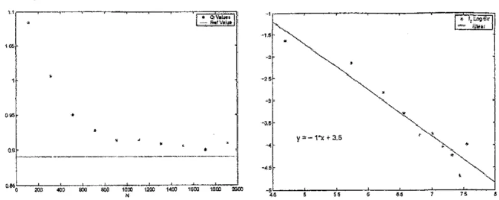
number $\overline{N}$ of pointsat eachtime grid.

4.1.1 Test 1 :

convergence

ofthe filter at a fixed instant

n

when the number

ofpoints $\overline{N}$ of each grid goes to infinity

The approximatefilter $\hat{\Pi}_{n}$ is computed

on the test functions $\phi_{i}$, i.e. $\Pi_{n}\phi:$, for $\phi_{1}(x)$ $=$ $x_{d}$, $x=(x_{1}, \ldots, x_{d})$

$\phi_{2}(x)$ $=$ $|x|^{2}$, $\phi_{3}$($) $=$ $\exp(-|x_{d}|)$,

in signal dimension $d=1$ _{and 3.} The following figures showthe

convergence

and the rate

of convergence of the approxim ated filter by quantization, when $\overline{N}$ goes to

infinity. The

theoretical convergencerate $\overline{N}^{\frac{1}{d}}$

(seeRemark 3.2) isthen in In-scale 1 in dimension 1 and

1/3in dimension 3, and is consistentto what

we

foundbynumericalexperiments. Actually,

we

even

get betterrateof

convergence

with the numerical tests.

Figure la: diml-:Convergence and Convergence Rate (ina$\ln$-scale) of$\hat{\Pi}_{n}\phi_{1}$ as$\mathrm{N}$ grows,

Figure lb : diml -: Convergence and Convergence Rate (ina $\ln$-scale) of$\hat{\Pi}_{n}\phi_{2}$ $\mathrm{f}\mathrm{f}\mathrm{i}$ $\mathrm{N}$ grows,

for$n=15$and $\phi_{2}(x)=x^{2}$.

Figure lc : diml -: Convergence and ConvergenceRate (in a$\ln$-scale) of$\dot{\Pi}_{n}\phi_{3}$ as $\mathrm{N}$grows,

for$n=15$ and $\phi_{3}(x)$$=\exp(-|x|)$

.

07 $00$ $-\sim-\mathrm{o}u’\acute{\mathrm{v}}\cdot \mathrm{t}\mathrm{u}\mathrm{v}\cdot\oe\cdot$

.

’ $-\mathrm{r}-\mathrm{i}$

.

$

―…

dotarrow–$

02 $0\mathrm{Q}$ $\mathfrak{N}$ $m$ $m$ $m$ {$\mathfrak{M}\mathrm{N}$

$\tau \mathrm{m}$ $m 1n _leeo rcoo

Figure $2\mathrm{a}$: dim3- : Convergence and Convergence Rate (ina$\ln$-scale) of$\hat{\Pi}_{7l}\phi_{1}$ as$\mathrm{N}$ grows,

92

$\mathrm{t}\infty$ $-\cdot*’ \mathrm{w}^{\mathrm{R}}\dot{\omega}0*|$ $*$

.

.

$\wedge$ $\mathrm{s}$ $A$

—-.

1

.

$\cdot$ —— $\mathrm{m}_{0}$

$xo$ $\mathrm{r}\mathrm{o}$ $\mathrm{g}w$ $\prime 0_{\mathrm{N}}oe\mathrm{t}\mathrm{I}\prime 4\infty 76\infty\backslash e\omega$ $\mathrm{m}$

Figure$2\mathrm{b}$ : dim3 -: Convergence and Convergence Rate (inaIn-scale)of$\hat{\Pi}_{n}\phi_{2}$ as$\mathrm{N}$ grows,

for$n=15$ and$\phi_{2}(x)$ $=|x|^{2}$

.

06

05

-$\cdot$

$\mathrm{R}\cdot 1\mathrm{V}*\mathrm{I}*0\cdot \mathrm{w}$

$–$. ——

$–=–.-$

.

$*$ $\mathrm{o}\mathrm{a}$ 0’ $0_{\mathfrak{g}}$ $2\Phi$ $4\infty$ $\epsilon\infty\iota\infty\tau_{\aleph}\mathrm{m}\prime \mathrm{T}\mathfrak{d}$

$\prime \mathrm{m}’\infty \mathrm{Q}\{\mathrm{o}\mathrm{m}2\mathrm{R}$

Figure$2\mathrm{c}$ : dim3 -: Convergence and Convergence Rate (in a In-scale) of$\hat{\Pi}_{n}\phi_{3}$ as $\mathrm{N}$grows,

for$n=15$ _and$\phi_{3}(x)=\exp(-|x_{3}|)$.

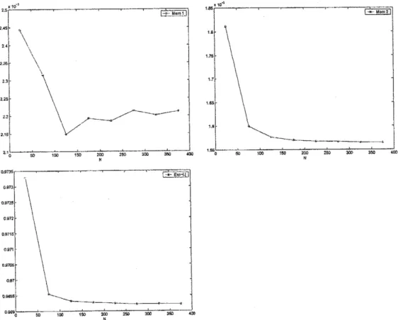
4.1.2 Test 2 : Stability ofthe filterfor

a

fixed grid size $\overline{N}$

as

n goes

to infinity.

We perform numerical tests for a signal in dimension 2. The following figures show the

stability of the quantized filter when thehorizon$n$ goes to infinity.

Figure3. $\dim 2-$ : Error_dependence of$\hat{\Pi}_{n}\emptyset$ as

$n$ grows,

4.2

A

stochastic

volatility

model

We

now

consider the

ARCH

model :

$X_{k+1}$ $=$ $pX_{k}+\epsilon_{k}$, $X_{0}\sim\nu N(0, \Sigma_{0})$

$Y_{k}$ $=$ $\sigma(X_{k})\eta_{k}$, $\sigma(x)=\gamma+|x|$,

where $(\epsilon k)$ are $(\eta_{k})$ independent Gaussian noises. This model is popular in finance, as

a discretization ofstochastic volatility model, where $X$ is the volatility and $Y$ the price

process. Unlike Kalman-Bucy model, there is

no

explicit reference formulafor the filter.

The following figures show the

convergence

of the quantized filterwhen$\overline{N}$ goes to infinity.

$0\theta 735$ $\mathrm{o}\mathrm{s}73$ $\mathrm{o}sr_{-}5$ $0972$ $0\mathrm{B}745$ $0\mathrm{B}7\mathrm{t}$ osm $0\mathrm{B}7$ oma

$\mathrm{o}s\mathrm{a}\mathrm{e}_{0}$ ₅₀ $’\infty$ $\infty$ $2\infty\aleph$

$2\mathfrak{B}$ $3\infty$ $\mathrm{g}$ $\mathrm{m}$

Figure 4:SVmodel:filtervalues of$\hat{\Pi}_{n}\emptyset$ at fixedn

as

$\overline{N}$grows,

for$\phi(x)=x$, $|x|^{2}$, and$\exp(-|x|)$.

More numerical illustrations

are

investigated in Sellami’s thesis [12] with in particular

comparison to Monte-Carloparticlemethods.

5Approximation

of the filter

process

by

quantization

In the quantization algorithm

described

in the previous section,

we

need for each

new

84

likelihoodobservationfunction$gk$

.

Thison-linephasemaybe

rem

ovedby

an

off-line

prepro-cessing ofthe observations, assuggested in [6], Onecanthenstoreinadditionto the signal

quantizers, the local likelihood functions precomputed onthesignal-observation grids. This

observation quantization approach is developed in [11],where errorestimation are provided

and numerically illustrated. If

we

stressthe dependence of the filter on the observation :

$\Pi_{n}(Y_{0}, \ldots , Y_{n})$, then it is approximatedby $\Pi\wedge n(\hat{Y}0$,.

.

.

,$\hat{Y}_{n})$, where $\hat{Y}_{k}$ is a quantizer of Yk.

However, wenoticethat the size ofthelook-up tables forthe filter may be

very

large. For

instance, if$\hat{Y}_{k}$

takes $M$values, then at time$n$,therandomfilter $\hat{\Pi}_{n}(\hat{Y}_{0}, . ., ,\hat{Y},)$ would take

$M^{n}$ values in $\mathcal{P}(E)$, which may explode for a long horizon $n$

.

This makes computations

untractable when solving dynamic optimization problems under partialinformation,

even

if$E$ is already afinitestate space

Inorder to

overcome

this numerical difficulty,

we

present

a

quantization approach

in-troduced in [9] and based

on

the Markov property ofthe pair filter-observation $(\Pi k, Y_{k})$

with respect to the observation filtration $(F_{k}^{Y})$

.

Indeed, by denoting $(\mathcal{F}_{k})$ the filtration

generated by $(X_{k}, Y_{k})$, and usingthe law ofiterated conditionalexpectations, we have for

any $k$ an$\mathrm{n}\mathrm{d}$ bounded Borelian function

$\varphi$ on $\mathcal{P}(E)\mathrm{x}$ $\mathbb{R}^{q}$ :

$\mathrm{E}[\varphi(\Pi_{k+1}, Y_{k+1})|F_{k}^{Y}]$

$=$ $\mathrm{E}[\mathrm{E}[\varphi(\overline{G}_{k+1}(\Pi k, Yk_{t}.Yk+1), Yk+1)|\mathcal{F}k]|F_{k}^{Y}]$

$=$ $\mathrm{E}$ $[ \int\varphi(\overline{G}_{k+1}(\Pi_{k}, Y_{k},y’), y’)P_{k+1}(X_{k}, dx’)qk+1(X_{k}, Y_{k}, x’, dy’)|F_{k}^{Y}]$

$=$ $\oint\varphi(\overline{G}_{k+1}(\Pi_{k}, Y_{k}, y’), y’)P_{k+1}(x, dx’)qk+1(x, Y_{k}, x’, dy’)\Pi_{k}(dx)$. (5.6)

This shows the Markov property of (Zk) with probability transition $R_{k}$ (from time $k-1$

to $k$) given by :

$R_{k}\varphi(\pi, y)$ $=$ $\int\varphi(\overline{G}_{k}(\pi, y, y^{\mathit{1}}), y’)Q_{k}(\pi,y, dy’)$, (5.7)

where$Qk(\pi, y, dy’)$is the law of$Yk$ conditional

on

$(\Pi k-1_{7}Yk-1)=(\pi, y)$with density :

$y’$ $arrow$ $\int gk(x, y, x’, y’)Pk(x, dx’)\pi(dx)$

.

We consider

a

framework with finitestate space : $E=\{x^{1}, \ldots, x^{m}\}$,

so

that the filter$\Pi_{k}$

is a random discreteprobability

measure

identified with

a

random vector$\Pi_{k}=(\Pi_{k}^{\tau})_{1\leq\not\in\leq m}$

in the simplex$K_{m}$ of$\mathbb{R}^{m}$ :

$K_{m}$ $=$ $\{\Pi\in \mathbb{R}_{+}^{m}$ : $\sum_{i=1}^{m}\Pi^{i}=1\}\simeq \mathcal{P}(E)$.

The idea is to apply

a

marginal quantization of theMarkov chain $(z_{k})=(\Pi k, Yk)$ valued

in$K_{m}\mathrm{x}$ $\mathbb{R}^{q}$. Hence, foreach $k=0$,

$\ldots$,$n$,

we

denote

$\hat{Z}_{k}$

the

associated

quantizer ontheoptimalgrid$zk=$ $(z_{k-}^{1}$,

. . .

,$z_{k}^{N_{k}})$ ofsize$N_{k}$points in$K_{m}\mathrm{x}\mathbb{R}^{q}$

.

Theprobability transition $R_{k}$ of the Markov chain (Zk) is approximated by the transition

matrix $\hat{R}_{k}=(\hat{r}_{k}^{\mathrm{z}j})$ :

$\hat{r}_{k}^{ij}$ _$=$ $\mathrm{P}$ _{$[\hat{Z}_{k}=z_{k}^{j}|\hat{Z}_{k-1}=z_{k-1}^{i}]$}.

The optimal grids $zk$ andtheassociated transition weights$\hat{r}_{k}^{ij}$

are

processed andestimated

bythe Kohonen algorithm. Thisis based

on

theMonte-Carlo simulationsof$(Z_{k})$, whichrely

themselves, from (5.7),

on

the followingsimulation procedure of theprobability transition

$R_{k}$ :

.

simulate$X_{k-1}$ with probabilitylaw $\Pi_{k-1}$, and then$X_{k}$ accordingto the probability

transition $P_{k}$

.

simulate $Y_{k}$ accordingto theprobability transition $\mathit{9}k(Xk-l, Yk-1, Xk)dy’$

.

compute$\Pi_{k}$ by theforward filtering (finite-dim ensional) equation

$\Pi_{k}$ $=$ $\overline{G}_{k}(\mathrm{I}\mathrm{I}_{k-1}Y_{k-1}, Y_{k})=\frac{\Pi_{k-}{}_{1}H_{k}}{\Pi_{k-}{}_{1}H_{k}(E)}$.

6

Application

:pricing

of

American options under

partial

observation

6.1

Optimal stopping problem under partial observation

Given

a

bounded measurablefunction $h$

on

$E\mathrm{x}$ $\mathbb{R}^{q}$, and

a

horizon

$n$,

we

denotefor any $k$

$=0$,$\ldots$,$n$, $T_{k,n}^{Y}$

as

theset of

$(F_{k}^{Y})$-stoppingtimes valuedin $\{k, \ldots, n\}$, and we consider the

following optimalstopping problem under partial observation :

$U_{k}$ $=$

$\mathrm{e}\mathrm{s}\mathrm{s}\sup_{\tau\in T_{\mathrm{t}^{Y}n}}.,\mathrm{E}[h(X_{\tau}, Y_{\tau})|F_{k}^{Y}]$

.

(6.8)

By usingthelawof iterated conditional expectation and the definition of thefilter,we notice

that problem (6.8)

may

bereduced to acompleteobservationmodel with state variable the

$(F_{k}^{Y})$-adaptedprocess (Zk) :

$U_{k}$ $=$

$\mathrm{e}\mathrm{s}\mathrm{s}\sup_{\tau\in \mathcal{T}_{k,n}^{Y}}\mathrm{E}$

$\ovalbox{\tt\small REJECT}\sum_{j=k}^{n}1_{\tau=j}\mathrm{E}[h(X_{j_{2}j}Y)|F_{j}^{Y}]|\mathcal{F}_{k}^{Y}\ovalbox{\tt\small REJECT}$

$=$ $\mathrm{e}\mathrm{s}\mathrm{s}\sup_{\tau\in \mathcal{T}_{k,n}^{Y}}\mathrm{E}\ovalbox{\tt\small REJECT}\sum_{\mathrm{i}=k}^{n}1_{\tau=j}\Pi_{\mathrm{J}}h(., Yj)|F_{k}^{Y}\ovalbox{\tt\small REJECT}$

$=$

$\mathrm{e}\mathrm{s}\mathrm{s}\sup_{\tau\in T_{k,n}^{Y}}\mathrm{E}$

$[ \Pi_{\tau}h(., Y_{j})|F_{k}^{Y}]=\mathrm{e}\mathrm{s}\mathrm{s}\sup_{\tau\in \mathcal{T}_{k_{J}n}^{Y}}\mathrm{E}[\tilde{h}(Z_{\tau})|F_{k}^{Y}]$,

with the notation :

se

By the $(F_{k}^{Y})$-Markov property of (Zk) and the dynamic programming principle,

we

have

$U_{k}=u_{k}(Zk)$ where functions$uk$ arecalculatedinbackward inductionby :

$u_{n}(z)$ $=$ $\tilde{h}(z)$

$u_{k}(z)$ $=$ $\max\{\tilde{h}(z)$ , $\mathrm{E}[u_{k+1}(Z_{k+1})|Z_{k}=z]\}$

.

Following [1],

we

provide a quantization approximation of $U_{k}=uk(Zk)$ by $\hat{U}_{k}$ =\^u$k(\hat{Z}k)$,

where $(\hat{Z}k)$ is a marginal quantization of $(Z_{k})$

on

grid _$zk$,

as

described in the previous

section, andfunctions $\text{\^{u}}_{k}$

are

explicitly computed

in

recursive form by :

$\hat{u}_{n}(z)$ $=$ $\overline{h}(z)$

$\hat{u}_{k}(z)$ $=$ $\max\{\overline{h}(z))\mathrm{E}[\hat{u}_{k+1}(\hat{Z}k+1)|\hat{Z}_{k}=z]\}$.

Proman algorithmic viewpoint, this reads as :

$\hat{u}_{n}(z_{n}^{i})$ _$=$ $\overline{h}(z_{n}^{i})$, $\mathrm{i}=1$,.

.

. ,$N_{n}$

$\text{\^{u}}_{k}(z_{k}^{i})$ $=$ $\max\{\overline{h}(z_{k}^{i}),$ $N \sum_{j=1}^{k+1}\hat{r}_{k+1}^{i\gamma}\hat{u}_{k+1}(z_{k+1}^{j})\}$ , $\mathrm{i}=1$,

$\ldots$,$N_{k}$

.

$L^{1}$-error estimation

||Uk--\^U

$k||_{1}$ in terms ofquantization

error

$||Z_{k}-\hat{Z}\iota.||_{2}$ is stated in [9],

6.2

Numerical illustration :

Bermudean options

in

a

partially

observed

stochastic volatility model

We consideran observablestock (logarithm) price $Y_{k}=$ in$s_{k}$, with dynamics given by :

$Y_{k+1}$ $=$ $Y_{k}+(r- \frac{1}{2}X_{k}^{2})\delta$ $+X_{k}\sqrt{\delta}\epsilon_{k+1}$

where $(\epsilon_{k})$ is a sequence ofGaussian whitenoise, and (Xk) is the unobservable volatility

process. $\delta=\frac{T}{n}$ is the time step from

an

Euler scheme.

We

assume

that $(X_{k})$ is

a

Markov

chain approximation

a

la Kushner [5] with spatial step

A

and with $m=3$ states of

a

mean-reverting

process

:

$dX_{t}$ $=$ $\lambda(x_{0}-X_{t})dt+\eta dW_{t}$

.

Inthiscontext ofapartially observed stochastic volatility model,

we

consider

a

Bermudean

put option with payoff$h(y)=(\kappa-e^{y})_{+}$, andwith price :

$u_{0}$ $=$ $\sup \mathrm{E}[e^{-r\tau \mathit{5}}h(Y_{\tau})]$ . (6.9)

$\tau\in \mathcal{T}_{0,n}^{Y}$

We perform numericaltests with :

-Price andputoption parameters : $r=0.05$, $S_{0}=110$

,

ts $=100$,

-Volatility param eters : A $=1$, _y7 $=0,1_{7}X_{0}=0.15$,

- Spatial step : _{$\Delta=0,05$}.

- Quantization :Grids

are

of

same

size $\overline{N}$ fixed for each time

$E[\Pi_{n}^{1}]$ $E^{\lceil}.\Pi_{n}^{2}]$ $E[\Pi_{n}^{3}]$ Relative

error

(%)

Monte Carlo 0.287608

0.422833

0.289558

Quant. with $\overline{N}=300$ 0.301651 0.421725 0.276624 $0.89\mathrm{S}$

Quant. with $\overline{N}=600$

0.301604 0.421458

0.276938 0.886

Quant. with $\overline{N}=900$

0.301598 0.421316

0.277086

0.881

Quant. with $\check{N}=1200$ 0.301618

0.42122

0.277162

0.879

Quant. with $\overline{N}=1500$ 0.301605 0.421205 0.27719 0.878

Table 1: Comparison ofquantized filter valueto its

Monte

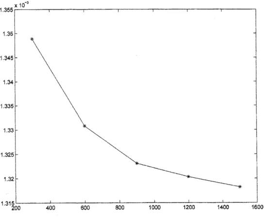
Carlo estimation

We first compare in Table 1 the filter expectation at the final date computed with

a

time stepsize $\delta$ $=1/5$ andbyusing the optim al quantization method withincreasinggrid

size$\overline{N}$ , andwith 10 Monte Carlo iterations,

Weobserve that besides the very low error level, the absolute error (plottedin Figure

5) and therelative

error are

decreasing

as

the gridsize grows.

Figure5: Filtererror convergenceas $\mathrm{N}$ grows

Secondly, in order to illustrate the effect of the time step,

we

compute the Anerican

option price under partial observation when the time step $\delta$ decreases to

zero

(i.e.

$n$

98

(Xk,$Y_{k}$). Indeed, in the limit for $\deltaarrow 0$

we

fully observe the volatility, and

so

the partial

observationpriceshould converge to the complete observation price.

Moreover, when we have more and more observations, the difference between the two

pricesshould decrease andconvergeto

zero.

This isshowninfigure6, where we performed

option pricing

over

grids of size $\overline{N}_{\Pi,Y}=1500$ in

case

of partial observation. The total

observation priceis given by the

same

pricing algorithm carried out

on

$\overline{N}_{X_{\rangle}Y}=45$ points

fortheproduct grid of$(Xk, Yk)$

.

For

fixed$n$, the rateof

convergence

for the approximation

ofthe value function under partial observation is oforder $\tilde{N}_{\Pi,Y}^{1/(m-1+d)}$ where $\overline{N}_{\Pi_{\mathrm{z}}Y}$ is the

number of points used at each time $k$ for the grid of$(\Pi k, Yk)$ valued in $K^{m}\mathrm{x}\mathbb{R}^{d}$

.

Prom

results of [1],

we

also know that therate of

convergence

for the approximation of the value

functionunderfull observationisoforder$m\mathrm{x}\overline{N}_{Y}$ where $\overline{N}_{X,Y}=m\mathrm{x}\overline{N}_{Y}$ is the number of

points ateach time$k$, usedforthe grid of_{$(Xk, Yk)$} valuedin$E\mathrm{x}\mathbb{R}^{d}$

.

This explains why, in order to have comparable results, and with$m=3$ and$d=1$,

we

have chosen $\overline{N}_{Y}\sim\overline{N}_{\Pi_{\mathrm{z}}Y}^{1/3}$

Figure6: Partial andtotal observation option pricesas$3arrow 0$

In addition, it is possible to observe the effect of information enrichment

as

the time

step decreases. In fact, if

we

considermultiples of$n$

as

the time step parameter,

we

notice

thatthe

American

option priceincreases forbothtotalandpartial observationmodels (see

4 8 16

Tot. Obs. $(\overline{N}_{X}‘ Y=30)$ 1.45863

1.75689 1.77642

Part. Obs. $(\overline{N}_{\mathrm{I}\mathrm{I},Y}=1000)$ 0.921729 1.13898 1.47089

Variation

0.53 0.61 0.30

Table 2: Am erican option price for embedded filtrations-First Example

Table 3: American option pricefor embedded filtrations- Second Example

References

[1] Bally V. and G. Pages (2003)

.

“A quantization algorithm for solving discrete time

multi-dimensional optimal stopping problems”, Bernoulli,9, 1003-1049.

[2] Elliott R., Aggoun L. and J. Moore (1995) : Hidden Markov models, estimation and control,

Springer Verlag

[3] Genon CatalotV. (2003) : “A nonlinear explicit filter”, Stat Prob. Lett, 61, 145-154.

[4] Stat S and H Luschgy (2000) : :Foundations

_of

quantization

_for

random $uectors_{)}$LectureNotes

in Mathem atics$\mathrm{n}^{0}1730$_,Springer, Berlin, 230 pp.

[5] Kushner H.J. and P. Dupuis (1992) . Numerical Methods

for

Stochastic Control Problems $m$

Continuous Time, Springer, NewYork

[6] Newton N. (2001) : “Approximations for nonlinear filters basedonquantization”, Monte Carlo

Methods and Appl, 7, 311-320.

[7] Pag\‘es G. and H. Pharn (2005) : “Optimal quantization methods for nonlinear filtering with

discrete-time $\mathrm{o}\mathrm{b}\mathrm{s}\mathrm{e}\mathrm{r}\mathrm{v}\mathrm{a}\mathrm{t}\mathrm{i}\mathrm{o}\mathrm{n}\mathrm{s}^{y}’$, Bernoulli, 11.

[8] Pages G,, Pham H. and J. Printems (2004) : “Optimal quantization methods and applications

tonumericalproblemsirrfinance”, Handbook

_of

computational andnumericalmethods infinance,

ed S. Rachev,Birkhauser.

[9] Pham$\mathrm{H}_{2}$. Runggaldier W. andA.Sellami (2005) : “Approximation by quantization of the filter

process and applications to optimal stopping problemsunderpartialobservation”, Monte Carlo

Methods andApplications, 11, 57-82.

[10] Sellami A. (2004) : “Nonlinear filtering with observation quantization”, Preprint, Laboratoire

deProbabilit\’esetmod\‘eles aleatoires, $\mathrm{U}\mathrm{n}\mathrm{i}\mathrm{v}\mathrm{e}\mathrm{r}\mathrm{s}\mathrm{i}\mathrm{t}\mathrm{e}^{J}\mathrm{s}$ Paris 6

&

7(France).

[11] Sellami A. (2005) : “Quantization based filtering method using first order approximation”,

Preprint PM A-1009.

[12] Sellami A. (2005) : Methodes de quantification optimaleen filtrage et appl cationsenfinance,