THE SPECTRAL FUNCTION AT A MAXIMUM OF THE POTENTIAL(Spectral and Scattering Theory and Related Topics)

THE SPECTRAL FUNCTION AT A

MAXIMUM

OF THE

POTENTIAL

IVANA ALEXANDROVA,_{JEAN-FRAN\cCOIS} BONY, AND THIERRYRAMOND

1. INTRODUCTION AND STATEMENT OF RESULTS

We studythestructureof thespectralfunction of theSchr\"odinger operatorwith shortrange

potential at an energy, whichisanon-degenerate maximumof the potential. We prove that it

is semi-classical Fourier integral operator quantizing the incoming and outgoing Lagrangian

submanifolds associated to the fixed hyperbolic point. We then give the oscillatory integral

representation of the spectral functionimplied by this result.

More precisely, we work in the following setting. We consider the operator

$P(h)=- \frac{1}{2}h^{2}\Delta+V,$ _{$0<h\ll 1$},

where $V\in C^{\infty}(\mathbb{R}^{n};\mathbb{R}),$ $n>1$, is a short range potential, i.e., for

some

_$\rho>1$ and all $\alpha\in N^{n}$

(1) $|\partial^{\alpha}V(x)|\leq C_{\alpha}(1+\Vert x\Vert)^{-\rho-|\alpha|},$ $x\in \mathbb{R}^{n}$

.

Then$P(h)$ admits

a

uniqueself-adjoint realization

on

$L^{2}(\mathbb{R}^{\mathfrak{n}})$with domain $H_{h}^{2}(\mathbb{R}^{n})$, the

semi-classical Sobolevspacesof order2 (see Appendix A). Denotingby$\{E_{\lambda}\}$ thespectralfamily of $P$,

we

shall

use

$e_{\lambda}$ for the Schwartz kernel of$E_{\lambda}$ for $\lambda>0$

.

The Limiting Absorption Principle

states that in $\mathcal{B}(L_{\alpha}^{2}(\mathbb{R}^{n}), L_{-\alpha}^{2}(\mathbb{R}^{n}))$ , where $L_{\alpha}^{2}(\mathbb{R}^{n})=\{f :f\langle\cdot\rangle^{\dot{\alpha}}\in L^{2}(\mathbb{R}^{n})\},$$\alpha>\Sigma 1$ the imit

$R( \lambda\pm iO, h)^{d}=^{of}\lim_{\epsilon\downarrow 0}(P(h)-(\lambda\pm i\epsilon))^{-1}$ for $\lambda>0$ exists.

We let $p(x, \xi)=\frac{1}{2}||\xi||^{2}+V(x)$ denote the principal symbol of$P(h)$ and denote its

Hamil-tonian vectorfield by $H_{p}= \sum_{j=1}^{n}(\ovalbox{\tt\small REJECT}_{j}\tau_{x_{j}}^{\partial_{--}}\#_{x_{j}}\pi_{f}^{\theta})$

.

Anintegral

curve

$\gamma$of$H_{p}$ will be called

a trajectory and will be denoted $\gamma(\cdot;x_{0},\xi_{0})$, if $(x_{0},\xi_{0})\in T^{*}\mathbb{R}^{n}$ are its initial conditions. We

recall that

Definition 1. The $trajecto\eta\gamma(\cdot;x_{0}, \xi_{0})$ is non-trapped

if

$\lim_{1arrow\pm\infty}||x(t;x_{0},\xi_{0})||=\infty$

.

The

$ene\eta y\lambda>0$ is non-trapping

if

for

every $(x_{0},\xi_{0})\in T^{r}\mathbb{R}^{n}$ with $l^{||\xi_{0}||^{2}}1+V(x_{0})=\lambda$ we have $\lim_{tarrow\pm\infty}||x(t;x_{0},\xi_{0})||=\infty$

.

We referto the $Append\dot{\alpha}$ for the relevant parts of semi-classical analysis used throughout

this paper.

The structure of the spectral function for Schr\"odinger-like operators has been studied

ex-tensively. Popov and Shubin [14], Popov [13], and Vainberg [18] have established high energy

asymptotics for thespectralfunction of secondorderelliptic operatorsunder the non-trapping

assumption.

Robert and Tamura [17] consider the spectral function for semi-claesical Sir\"odinger

oper-ator with short range potentials and establish asymptotic expansions at fixed non-trapping

and non-critical trapping energies in the

sense

of

a

distribution.

The microlocal structureof the spectral function has also been analyzed. In [19, $Th\infty rem$

XII.5] Vainberg establishes

a

high energy asymptotic expansion ofthe spectral function for

compactly supported smooth perturbations of the Laplacian assuming that the $ener_{\Psi}1$ is

non-trapping. This asymptotic expansionis expressed this in theformof

a

Maslov canonical operator $K_{\Lambda,\lambda}$ associated to

a

certain Lagrangiansubmanifold$\Lambda=\Lambda_{y}\subset T^{*}\mathbb{R}^{\mathfrak{n}}$and acting

on

another asymptotic sumin $\lambda$

.

The Lagrangian submanifold $\Lambda_{y}$ consists ofthe phsse

trajecto-ries atenergy 1 of the principal symbol of$A$passing throughafixed base point$x(O)=y$,while

the terms of the asymptotic sum

on

which $K_{\Lambda,\lambda}$ acts solve a recurrent system oftransport)

equations along the phase trajectories ofthe system.

GerardandMartinez [10]

prove

thatthe spectralfunctionfor certain long-rangeSir\"odinger

operators at non-trapping energies $\lambda$ is a semi-classical Fourier integral operator (h-FIO)

associated to $( \bigcup_{t\in R}$graph$\exp(tH_{p})|_{p^{-1}(\lambda)})’$

.

Near the diagonal $\{(x,\xi;x,\xi) : p(x,\xi)=\lambda\}$ they

also give the following oscillatory integral representation of the spectral function

$e_{\lambda}(x,y, \lambda, h)\equiv\frac{1}{(2\pi h)^{n}}\int_{S^{\mathfrak{n}-1}}e^{i}\pi^{\varphi(x,y\rho,\lambda)}a(x,y,\omega, \lambda)\ )$

where $\varphi$ is such that $(\partial\#_{x})^{2}+V(x)=\lambda$ and $\#_{x}^{\partial}|_{(x-y,w)=0}=\sqrt{\lambda-V(x)}\omega,$ $\varphi|_{x\approx y}=0$

.

In [1] the first author has proven that the spectral function restricted away bom the

di-agonal in $\mathbb{R}^{n}x\mathbb{R}^{n}$ at non-trapping energies, and at trapping energies under the absence

of

resonances

near the real axis, is an h-FIO associated to $( \bigcup_{t=0}^{T}$graph$\infty(tH_{p})|_{p^{-1}(\lambda)})’\cup$

(

$\bigcup_{t=0}^{-T}$graph

$\infty(tH_{p})|_{p^{-1}(\lambda)}$

)

for

some

$T>0$

near a

non-trapped trajectory. Under

a

function of the form

$e_{\lambda}(x,y, \lambda)\equiv\int e^{i}\pi^{S(x,y,t)}a(x,y,t)dt$,

where $S(x,y,t)= \int_{l(t,x,y)}\frac{1}{2}\Vert\xi(t)\Vert^{2}-V(x(t))+\lambda dt$is the action

over

the segment $l(t,x,y)$ of

the trajectorywhich connects $x$ with $y$ at time $t$ and $a\in S_{2n+1}^{+}(1)n8$

Hassell and Wunsch [11] have studied the structure of the spectral function on $\infty mpact$

manifolds with boundary equipped with scattering metrics. Their result roughly says that

the spectral function is

an

intersecting Legendrian distribution.

Here

we

studythestructureofthespectralfunctionunderthe following additional

assump-tions:

(A1) $V$ has

a

non-degenerate global maximum at $x=0$, with $V(O)=E>0$ and

$V(x)=E- \sum_{j=1}^{n}\frac{\lambda_{j}^{2}}{2}x_{j}^{2}+O(x^{3}),$ $xarrow 0$

,

where $0<\lambda_{1}\leq\lambda_{2}\leq\ldots\leq\lambda_{\mathfrak{n}}$

.

(A2)

_{

$(x,\xi)\in p^{-1}(E)$ ; exp$(tH_{p})(x,\xi)-\neq\infty\dot{a}starrow\pm\infty$

}

$\equiv\{(0,0)\}$

Then the linearized vector field of$H_{p}$ at $(0,0)$ is

$d_{(0,0)}H_{p}=(\begin{array}{llll}0 Idiag(\lambda_{l}^{2} \cdots \lambda_{n}^{2}) 0\end{array})$

.

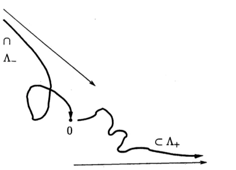
Therefore, by the Stable Manifold Theorem, there exist Lagrangian submanifolds $\Lambda\pm\subset$

$T^{*}\mathbb{R}^{\mathfrak{n}}$ satisfying

$\Lambda\pm=$

{

$(x,\xi)\in T^{*}\mathbb{R}^{n}$ : exp$tH_{p}(x,\xi)arrow(0,0)$

as

$tarrow\mp\infty$

}

(see Figure 1).

To state our main theorem, we further recall

&om

[12] that if $\rho\pm\in\Lambda\pm and\gamma\pm(\cdot;\rho\pm)=$

$(x\pm(\cdot;\rho\pm),\xi\pm(\cdot;\rho\pm))def=\gamma(\cdot;\rho\pm)$, then for some $g\pm\in c\infty(\mathbb{R}^{2n})$ and $\epsilon>0,$ $x\pm(t;\rho\pm)=$

$g\pm(\rho\pm)e^{\pm\lambda_{1}t}+O(e^{\pm(\lambda_{1}+e)t})$

as

$tarrow\mp\infty$

.

We let $\tilde{\Lambda}\pm=\{(\dot{x},\xi)\in\Lambda\pm:g_{-}(x,\xi)=0\}$and recall from [7] that dim$\tilde{\Lambda}\pm=n-m$, where $m^{d}=^{\epsilon f}\#\{j :\lambda_{1}=\lambda_{j}\}$

.

FIGURE 1. The incoming A-andoutgoing $\Lambda_{-}Lagr\mathfrak{U}1\dot{i}^{an}$ submanifolds.

Our main result is the following

Theorem 1. Micrvloeally near $(\rho+,\rho_{-})\in\Lambda+\backslash \tilde{\Lambda}_{+}(\rho_{-})x\Lambda_{-}\backslash \tilde{\Lambda}_{-}$, the resolvent$R(E+i0)\in$

$\mathcal{I}_{h}^{1-\frac{\Sigma_{j=1^{\lambda_{j}}}^{n}}{2\lambda_{1}}}(\mathbb{R}^{2n},\Lambda+x\Lambda_{-})$

.

Simdarly, microlocally

near

$(\rho-, \rho_{+})\in\Lambda_{-}\backslash \tilde{\Lambda}_{-}(\rho_{+})x\Lambda+\backslash \tilde{\Lambda}+$, the msolvent$R(E-iO)\in$

$\mathcal{I}_{\hslash}^{1-\frac{\Sigma_{j-1}^{n}\lambda_{j}}{2\lambda_{1}}}(\mathbb{R}^{2n}, \Lambda_{-}x\Lambda_{+})$

.

Remark. If$\lambda_{2}>\lambda_{1}$, then $\tilde{\Lambda}+(\rho_{-})=\tilde{\Lambda}+and$

$R(E+i0)\in \mathcal{I}_{h}^{1-\frac{\Sigma_{j--1}^{n}\lambda_{j}}{2\lambda_{1}}}(\mathbb{R}^{2n},\Lambda+\backslash \tilde{\Lambda}_{+}x\Lambda_{-}\backslash \tilde{\Lambda}_{-})$

.

The structure of the resolvent in various settings has been studied in [3], [4], and [11].

IFbr compactly supported and short range potentials, the resolvent has been shown to be a

h-FIO associated to the Hamiltonian flow relation of theprincipal symbol of$P\dot{r}estricted$ to

the

energy

surface in [3] and [4]. Hassell and Wunsch [11] identify theSchwartz kernel of the resolvent

on

a compact scattering manifold with aLegendrian distribution.

$U_{S\dot{i}}g$ Stone’s formula

$\frac{dE_{\lambda}}{d\lambda}(E)=\frac{1}{2\pi i}(R(E+iO)-R(E-iO))$,

we now

easily obtain from$Th\infty rem1$ the following

Corollary 1. Microlocally

near

$(\rho-, \rho_{+})\in\Lambda-\backslash \tilde{\Lambda}_{-}x\Lambda+\backslash \tilde{\Lambda}_{+}(\rho_{-})$, the spectml

function

$e_{B}\in \mathcal{I}_{h}^{1-\frac{\Sigma_{j--1}^{n}\lambda_{j}}{2\lambda_{1}}}(\mathbb{R}^{2n},\Lambda_{+}x\Lambda_{-})$

.

Microlocally

near

$(p+,\rho_{-})\in\Lambda+\backslash \tilde{\Lambda}_{+}x\Lambda_{-}\backslash \tilde{\Lambda}_{-}(\rho+)$, the $SpeCt\mathfrak{w}l$

function

$e_{B}\in \mathcal{I}_{h}^{1-\frac{\Sigma_{j--1}^{n}\lambda_{j}}{2\lambda_{1}}}$

(

$\mathbb{R}^{2n}$,A-x $\Lambda_{+}$

).

We

now

introduce

some

ofthe notation we $sha\mathbb{I}$

use

below. For a sequentially continuous

operator$W$ : $C_{c}^{\infty}(\mathbb{R}^{m})arrow \mathcal{D}’(\mathbb{R}^{n})$

we

shall denoteby$K_{W}$ itsSchwartz kernel. Onany smooth

man迂old $M$ we denote by $\sigma$ the canonical symplectic form

on

$T^{*}M$ and everywhere below

we work with the canonical symplectic structure on $T^{\cdot}M$

.

If_{$C\subset T^{*}M_{1}xT^{*}M_{2}$}, where $M_{j}$,

$j=1,2$

,

are smooth manifolds, we will use thenotation $C’=\{(x,\xi;y, -\eta) : (x,\xi;y,\eta)\in C\}$

.

We also set $B(O,r)=\{x\in \mathbb{R}^{n} : \Vert x\Vert<r\}$

.

We prove

our

main theorem in Section 2 and in Section 3

we

give the microlocal represen-tation of the spectral function implied by Theorem 1.

2. THE RESOLVENT AS A SEMI-CLASSICAL FOURIER INTEGRAL OPERATOR

Here weprove Theorem 1.

The resolvent estimate from [5, Theorem 2.1], $||R(E\pm i0)||_{\mathcal{B}(L_{\alpha}^{2}(B^{n}),L_{-\alpha}^{2}(B^{n}))}=O(*)$ ,

for $\alpha>\frac{1}{2}$ and [4, Lemma 1] give that $K_{R(B\pm i0)}\in \mathcal{D}_{h}’(\mathbb{R}^{2n})$

.

Let

$r_{\pm}(R, d, \sigma)=\{(x,\xi)\in \mathbb{R}^{n}x\mathbb{R}^{\mathfrak{n}}$: $||x||>R,$$\frac{1}{d}<||\xi||<d,$$\pm coe(x,\xi)>\pm\sigma\}$

with$R>1,$ $d>1,$ $\sigma\in(-1,1)$, and$\cos(x,\xi)=\ovalbox{\tt\small REJECT}_{x\xi}^{x}$, bethe outgoing andincomin$g$ subsets

ofphase space, respectively. We choose $d>0$ such that $\partial 1<E<d$

.

Let $u_{-}\in \mathcal{D}_{h}’(\mathbb{R}^{n})$ be such that $MS(u_{-})\subset\Gamma_{-}(R,d, \sigma)$ is $\infty mpact$, where $MS$ denotes its

microsupport.

We shall prove that $u=\cdot R(E+i0)u$-solves the problem

$\{\begin{array}{l}(P-E)u=0(0,0)u=\pi i_{\int_{0^{ee^{-}}}^{\tau::}dtu_{-}}\kappa^{tB}\pi^{tP}\Gamma_{-}(R,d,\sigma)\end{array}$

for

some

$T>0$ sufficiently large.

For the second condition, let $w-\in S_{2n}^{0}(1)$ have compact support and observe that for any

$T>0$

$w_{-}(x, hD_{x})R(E+i0)u_{-}=w_{-}(x, hD_{x}) \frac{i}{h}\int_{0}^{T}e^{\pi^{tE}}e^{-\pi^{tP}}dtu_{-}:$:

$+e\overline{h}w_{-}(x, hD_{x})R(E+i0)e^{-\pi^{TP}}u-:_{TE}i$

For the second term, observe that, by [5, Lemma 5.1] there exist $\sigma+\in(0,1)$ and $T_{0}>0$

suchthat for$T>T_{0}$

$MS(e^{-\neq P}:u_{-)}\subset T^{*}B(0,$$\frac{R}{2})\cup\Gamma+(\frac{R}{2},d,\sigma+)$

.

Let, now, $w+\in S_{2n}^{0}(1)$ have $\infty mp\epsilon ct$ support in $r_{+}(\frac{R}{3},d_{1},\overline{\sigma}_{+})$ for

some

$d_{1}>d$ and

$\overline{\sigma}+<\sigma+withw+=1$

on

$MS(e^{-\neq P_{u_{-)}}}i nr_{+}(\frac{R}{2},d,\sigma_{+})$ and let $\chi\in C_{c}^{\infty}(\mathbb{R}^{n})$ be such that

$\chi\equiv 1$ on$B(0, FR)$

.

Then two consecutive applicationsof [16, Lemma 2.3] give

$w_{-}(x, hD_{x})R(E+i0)e^{-\pi^{TP}}u_{-}$:

$=w_{-}(x, hD_{x})R(E+i0)\chi e^{-\pi^{TP}}u_{-}:+w_{-}(x, hD_{x})R(E+i0)w_{+}(x, hD_{x})e^{-\pi^{TP}}ui$一

$+O(h^{\infty})$

$=\mathcal{O}(h^{\infty})$

.

Thesame proof

as

of [5, Lemma 5.1]

now

gives that for $R>0$ sufficiently large,

we

have

that $\Lambda\pm\cap T^{*}(\mathbb{R}^{n}\backslash B(0,7R))\subset r_{\pm}(_{7}^{R}, d, \sigma\pm)$

.

Therefore, by [7, Theorem 2.6] and [7, Remark $2.\eta$, if $Op_{h}(a_{\pm})$ have compact wavefront sets in $r_{\pm}(_{T}^{R}, d, \sigma\pm)$

near

$p\pm$, respectively, then

microlocally

near

$(\rho+, \rho_{-})\in\Lambda+\backslash \tilde{\Lambda}_{+}(\rho_{-})x\Lambda_{-}\backslash \overline{\Lambda}_{-}$,

(2)

$Op_{h}(a_{+})R(E+i0)Op_{\hslash}(a_{-}) \equiv Op_{h}(a_{+})\mathcal{J}(E)\frac{i}{h}\int_{0}\tau_{::}e^{\pi^{tE}}e^{-}\pi^{tP}dtOp_{h}(a_{-})$,

if supp$a+is$ close to $(0,0)$

$Op_{h}(a_{+})R(E+i0)O p_{h}(a_{-})\equiv e^{-\frac{:}{h}s(P-B)}\dot{O}p_{h}(a_{+,\epsilon})\mathcal{J}(E)\frac{i}{h}$

。

$\tau_{::l ’ eT^{tE}e^{-\pi^{tP}}dte\kappa^{\iota(P-B)}Op_{h}(a_{-})}$

if $suppa+is$far from $(0,0),s>0$ islarge enough,

and $ess- supp_{h}a+,\delta\subset\exp(-sH_{p})$ess-supp$ha+$

where microlocaily

near

$(\rho+’ p_{-})\in\Lambda+\backslash \tilde{\Lambda}_{+}(\rho_{-})x\Lambda_{-}\backslash \tilde{\Lambda}_{-},$

$J(E)\in \mathcal{I}_{h}^{-\frac{\Sigma_{j-1}^{n}\lambda_{j}}{2\lambda_{1}}}(\mathbb{R}^{2n}, \Lambda_{+}xA_{-})$

.

Lemma 1. $\frac{i}{h}\int_{0^{e\pi^{tE}e^{-\frac{:}{h}tP}dt}}^{\tau:}\in \mathcal{I}^{\frac{1}{h2}}(\mathbb{R}^{2n}, \Lambda_{E}(R))$ ,

where

$\Lambda_{B}(R)=(\bigcup_{t>0}$graph exp$(tH_{p})|_{p^{-1}(E)})’$

.

Proof.

We recall the well known fact that $e^{-\not\in sP}\in \mathcal{I}_{h}^{0}$

(

$\mathbb{R}^{2n}$,(graph

$\infty(sH_{p})$)

)

for $s\in R$

.

For

$t$ sufficiently small we further have from [15, Proposition IV-14]

(3) $\dot{K}_{-,e*t(P-B)}=\frac{i}{(2\pi h)^{n}}\int_{R^{n}}e^{\pi^{(\varphi(\iota.x.\theta)-y\cdot\theta+tB)}}a(x,y, \theta)d\theta:$

,

where$\varphi\in C^{\infty}(\mathbb{R}^{2n+1})$satisfies$\varphi_{\iota}’+p(x, \varphi_{x}’)=0$ and $(x,\nabla_{x}\varphi(t,x, \theta))=\exp(tH_{p})(\nabla_{\theta}\varphi(t,x,\theta),\theta)$ ,

and $a\in s3.(1)$

.

We

now use

the following result, the proof ofwhich we postpone until later. Lemma 2. Let $\chi\in C_{c}^{\infty}(\mathbb{R})$

.

Then

$\frac{i}{h}\int_{0}^{\infty)}\chi(t)e^{-\pi^{t(P-B)}}dt\in \mathcal{I}_{h}^{I}(\mathbb{R}^{2n},\Lambda_{B}(R))$

.

Let, now, $\chi\in C_{c}^{\infty}(\mathbb{R}^{n})$ have support

near

$0$ and satisfy $\sum_{l\in\epsilon Z}\chi(t-l)=1$ for $t\in \bm{R}$ and

some

$\epsilon>0$ sufficiently small. Then

$\frac{i}{h}\int_{0}^{T_{i}}e^{-\pi^{t(P-B)}}dt=\frac{i}{h}\int_{0}^{T}\sum_{l\in\epsilon Z}\chi(t-l)e^{-\pi^{t\langle P-E)}}:dt=\frac{i}{h}\sum_{l\in \mathbb{Z}}\int^{T+l}\chi(s)e^{-}\pi^{\epsilon(P-B)^{i}}dse^{-\pi^{l(P-B)}}i$

It is

now

easy to

see

that the manifolds

$\Lambda_{E}(R)’x_{i}aph\exp(tH_{p})$

and

$T^{*}\mathbb{R}^{n}x$ diag$(T^{*}\mathbb{R}^{n}xT^{*}\mathbb{R}^{n})xT^{*}R^{n}$

intersect transverselyand therefore

$\frac{i}{h}\int_{0}^{T}\pi^{t(P4)}:$

.

口

We now return to the analysisof (2), It is easy to

see

that the manifolds

$\Lambda_{+}x\Lambda_{-}’x\Lambda_{B}(R)’$

and

intersect cleanly with excess 1 and from (2) and [9] we then have that microlocally near

$(p+,\rho_{-})\in\Lambda+\backslash \overline{\Lambda}_{+}(p_{-})x\Lambda_{-}\backslash \overline{\Lambda}_{-},$

$R(E+i0)\in \mathcal{I}_{h^{-\dot{r}_{\frac{--1^{\lambda}j}{2\lambda_{1}}}^{n}}}^{1^{\Sigma}}(\mathbb{R}^{2n},\Lambda_{+}\backslash \tilde{\Lambda}_{+}(\rho_{-})\cross\Lambda_{-}\backslash \tilde{\Lambda}_{-})$

.

The second part of the theorem is proven analogously.

Pmof of

Lemma

2.

As in (3)

we

have

$\frac{i}{h}\int\chi(t)e^{-\pi^{t(P-E)}}dt=\frac{i}{(2\pi)^{\mathfrak{n}}h^{\mathfrak{n}+1}}\int_{0}^{\infty}\int_{R^{n}}\chi(t)e^{-\frac{i}{h}(\varphi(t\rho,\theta)-y\cdot\theta+tB)}a(t,x,y,\theta)d\theta dt$

.

We shall prove that $\Phi(x, y;t, \theta)^{d}=^{of}\varphi(t,x,\theta)-y\theta+tE$is anon-degenerate phasefunction.

Let

$C_{\Phi}^{d}=^{ef}\{(x,y,t, \theta)\in \mathbb{R}^{3n+1} : \nabla_{\ell,\theta}\Phi(x,y;t, \theta)=0\}$

$=\{(x,y,t, \theta)\in \mathbb{R}^{3n+1} : \varphi_{t}’(t,x,\theta)=-E, \nabla_{\theta}\varphi(t,x,\theta)=y\}$ and for $(x, y,t, \theta)\in C_{\Phi}$ consider

$\{\begin{array}{l}d\Phi_{t}’d\Phi_{\theta}\end{array}\}(x,y;t, \theta)=\{\begin{array}{llll}\Phi_{tx}’’ \Phi_{ty}’’ \Phi_{tt}’’ \Phi_{t\theta}’’\Phi_{\theta x}’’ \Phi_{\theta y}’’ \Phi_{\theta t}’’ \Phi_{\theta\theta}’’\end{array}\}(x,y;t, \theta)=\{\begin{array}{llll}\varphi_{tx}’’ 0 \varphi_{u}’’ \varphi_{t\theta}^{jj}\varphi_{\theta x}’ I \varphi_{\theta t}’ \varphi_{\theta\theta}’’\end{array}\}(x,y;t,\theta)$

The bottom $n$ rows in the above matrix

are

clearly linearly independent. The last

row

is

never$0$for$(x,y,t, \theta)$ suchthat$\varphi_{t}(t,x,\theta)=-E=-p(x,\varphi_{x}(t,x, \theta))$ because from Assumption

2 it $f_{0}nows$ that $dp\neq 0$

on

$\{p=E\}\backslash \{(0,0)\}$

.

Therefore $d\Phi|c_{l}$ has maximum rank and $\Phi$ is

anon-degenerate phase function. This impliesthat $\pi^{\int_{0}^{T}e^{-\dot{f}^{t(P-B)}}dt}i$ is an h-FIO associated

to

$\Lambda_{\Phi}^{d}=^{\epsilon f}\{(x,\nabla_{x}\Phi(x,y;t, \theta);y,\nabla_{y}\Phi(x,y;t, \theta)) : (x,y;t,\theta)\in C_{\Phi}\}$

$=\{(x, \nabla_{x}\varphi(t,x,\theta);y, -\theta) : (x,y;t, \theta)\in C_{\Phi}\}=\Lambda_{B}(R)$

.

Ftom $[2, Th\infty rem2]$ we obtain that the orderof this h-FIO is $\frac{1}{2}$

3. MICROLOCAL REPRESENTATION OF THE SPECTRAL FUNCTION

Here

we

present the repr sentation of the spectral function

as

an oscillatory integral op-erator

near

Microlocally

near

$(\rho_{+}, p_{-})\in\Lambda+\backslash \tilde{\Lambda}_{+}(\rho_{-})x\Lambda_{-}\backslash \tilde{\Lambda}_{-}$

.

The osffiatory integral

representationnear $(p_{-},p_{+})\in\Lambda-\backslash \tilde{\Lambda}_{-}(p_{+})\cross\Lambda+\backslash \tilde{\Lambda}_{+}$ is analogous.

Theorem 2. Let $(\rho+, \rho_{-})\in\Lambda+\backslash \tilde{\Lambda}_{+}(\rho_{-})x\Lambda-\backslash \tilde{\Lambda}_{-}$

.

Then there exists a non-degenemte phase

_function

$\Psi\in C^{\infty}(\mathbb{R}^{2\mathfrak{n}+m})$ and a symbol $b\in$ $S_{2n+}^{1-\frac{\Sigma_{j--1}^{n}\lambda_{j}}{m2\lambda_{1}}+\oplus+\tau}(1)n$

such that microlocaily

near

$(\rho+, \rho_{-})$ $e_{B} \equiv\int_{R^{m}}e^{\frac{i}{h}\Psi(x,y,\tau)}b(x,y,\tau)d\tau$

.

Proof.

The assertion of the theorem follows $bom$ [$2$, Theorem 1] and Theorem 1. _口

Remark. If $(\rho+’\rho_{-})\in\Lambda+\backslash \tilde{\Lambda}_{+}(\rho_{-})x\Lambda_{-}\backslash \overline{\Lambda}$-are such that the projection from

$T^{*}\mathbb{R}^{n}$ to the base $\mathbb{R}^{n}$ restricted to $\Lambda\pm is$ a diffeomorphism in some neighborhoods of $\rho\pm$,

we

have $Rom$ [$6$, Theorem 46.$D$] that

near

$\beta\pm,$ $\Lambda\pm=\{(x,d_{x}S_{+}(x);y,d_{y}S_{-}(y))\}$, where

$s_{\pm}= \int_{\gamma\pm(\rho\pm)5}^{1}\Vert\xi\pm(t)||^{2}-V(x\pm(t))dt$

are

the actions

over

the half-trajectories $\gamma\pm(\rho\pm)=$ $(x\pm,\xi\pm)\subset\overline{\Lambda}\pm$ which start at $p\pm \bm{t}d$ approach $(0,0)$

as

$tarrow\mp\infty$

.

Therefore, Rom [2,

Theo-rem

1]

we

have that thereexist $b\in S_{2\mathfrak{n}}^{1.-\frac{\Sigma_{\dot{g}=1}^{n}\lambda_{j}}{2\lambda_{1}}+\frac{n}{2}}(1)$

such that

$e_{B}\equiv e^{i}\pi^{(s_{+}+S_{-})}b$microlocally

near

$(p+,\rho_{-})\in\Lambda+\backslash \tilde{\Lambda}_{+}(\rho_{-})x\Lambda_{-}\backslash \tilde{\Lambda}_{-}$

.

APPENDIX A. ELBMENTS OF SEMI-CLASSICAL ANALYSIS

Inthis section

we

recall

some

of theelementsof semi-classical analysiswhich

we

use

inthis

paper. First

we

recall the definitions of the$follow\dot{i}g$ two classes ofsymbols

$S_{2n}^{m}(1)=\{a\in C^{\infty}(\mathbb{R}^{2n}x(0, h_{0}])$ :$\forall\alpha,$$\beta\in N^{n},$$|\partial_{x}^{\alpha}\partial_{\zeta}^{\beta}a(x,\xi;h)|\leq C_{\alpha,\beta}h^{-m}\}$ and

$S^{m,k}(T^{*}\mathbb{R}^{n})=\{a\in C^{\infty}(T^{s}\mathbb{R}^{n}x(0, h_{0}])$ :$\forall\alpha,\beta\in N^{\mathfrak{n}},$ $|\partial_{x}^{\alpha}\partial_{\xi}^{\beta}a(x,\xi;h)|\leq C_{\alpha,\beta}h^{-m}\langle\xi)^{k-|\beta|}\}$,

where$h_{0}\in(0,1$] and $m,$$k\in R$

.

For $a\in S_{2n}^{m}(1)$ or $a\in S^{m,k}(T^{*}\mathbb{R}^{\mathfrak{n}})$

we

define the

correspond-ing semi-classical pseudodifferentialoperatorof class $\Psi_{h}^{m}(1,\mathbb{R}^{\mathfrak{n}})$ or $\Psi_{h}^{m,k}(\mathbb{R}^{n})$, respectively, by

setting

$Op_{h}(a)u(x)= \frac{1}{(2\pi h)^{n}}\int\int e*\perp x-\mu_{a}(x,\xi;h)u(y)dyd\xi,$ $u\in S(\mathbb{R}^{n})$ ,

and extending the definition to$S’(\mathbb{R}^{\mathfrak{n}})$ by duality (see [8]). Here we work only with symbols

which admit asymptotic expansions in $h$ and with pseudodifferential operators which

are

quantizations of such symbols. For $A\in\Psi_{\hslash}^{k}(1,\mathbb{R}^{\mathfrak{n}})$

or

$A\in\Psi_{h}^{m,k}(\mathbb{R}^{n})$,

we

shall

use

$\sigma_{0}(A)$ and $\sigma(A)$ to denote its principal symbol and its complete $8ymbol$, respectively. A semi-classical

pseudodifferential operator is said to be ofprincipal type if its principalsymbol$a_{0}$ satisfies

For $a\in S^{m,k}(T^{*}\mathbb{R}^{n})$

or

$a\in S_{2n}^{m}(1)$

we

define

ess-supp$h$$a$

$=\{(x,\xi)\in T^{*}\mathbb{R}^{n}|\exists\epsilon>0\partial_{x}^{\alpha}\partial_{\xi}^{\beta}a(x’,\xi’)=O_{C(B((x,\xi),e))}(h^{\infty}),$ $\forall\alpha,\beta\in N^{n}\}^{c}$

$\cup(\{(x,\xi)\in T^{*}\mathbb{R}^{\mathfrak{n}}\backslash \{0\}|\exists\epsilon>0\partial_{x}^{\alpha}\partial_{\xi}^{\beta}a(x’,\xi’)=O(h^{\infty}\langle\xi)^{-\infty})$ ,

uniformly in $(x’,\xi’)$ such that $||x-x’||+ \frac{1}{||\xi||}+\Vert\frac{\xi}{||\xi||}-\frac{\xi’}{||\xi||}\Vert<\epsilon\}/\bm{R}+)^{c}$

欧$T^{*}\mathbb{R}^{\mathfrak{n}}uS^{*}\mathbb{R}^{\mathfrak{n}}$,

where

we

define $S^{*}\mathbb{R}^{n}=(T^{*}R^{\mathfrak{n}}\backslash \{0\})/\mathbb{R}_{+}$and denoteby $\bullet^{c}$ the complement

of the set $\bullet$

.

For

$A\in\Psi_{\hslash}^{m,k}(\mathbb{R}^{\mathfrak{n}})$,

we

then define

$WF_{h}(A)=es$ -supp$h^{a,A}=Op_{h}.(a)$

.

We alsodefinetheclass of semi-classical distributions$\mathcal{D}_{h}’(\mathbb{R}^{\mathfrak{n}})$ withwhichwe willwork here

$\mathcal{D}_{\hslash}’(\mathbb{R}^{n})=\{u\in 0_{h}\infty((0,1];\mathcal{D}’(\mathbb{R}^{n}))$ : $\forall\chi\in c_{c}\infty(\mathbb{R}^{n})\exists N\in N$and _{$C_{N}>0$} : $|\mathcal{F}_{h}(\chi u)(\xi)|\leq C_{N}h^{-N}\langle\xi\rangle^{N}\}$

where

$\mathcal{F}_{h}(\chi u)(\xi)=\langle e^{-\pi^{\langle\cdot,\xi\rangle}}\ell,\chi u\rangle$,

and $\langle\cdot, \cdot\rangle$ denotes the distribution pairing. We also extend _{$thi_{8}$} definition in the obvious way

to $\mathcal{E}_{\hslash}’(\mathbb{R}^{n})$

.

The$L^{2}-baeed$ _{semi-classical Sobolev spaces $Hn(R^{n}),$ $s\in R$}, _which$\infty nsist$ of the

distribu-tioo $u\in \mathcal{E}_{\hslash}’(\mathbb{R}^{n})su\bm{i}$that $||u||_{H_{\dot{h}}(R^{n})}^{2^{d}}=^{of} \frac{1}{(2\pi\hslash)^{n}}\int_{R^{n}}(1+||\xi||^{2})^{\epsilon}|\mathcal{F}_{\hslash}(u)(\xi)|^{2}d\xi<\infty$

.

For $u\in \mathcal{D}_{h}’(\mathbb{R}^{n})$ we also defineits finite semi-classical wavebont set asfollows.

Deflnition 2. Let $u\in \mathcal{D}_{h}’(\mathbb{R}^{n})$ and let $(x_{0},\xi_{0})\in\tau*(\mathbb{R}^{n})$

.

Then the point $(x_{0},\xi_{0})$ does not

belong to $WF_{h}^{f}(u)$

if

the$r\epsilon$ esist

X $\in C_{c}^{\infty}(\mathbb{R}^{n})$ unth$\chi(x_{0})\neq 0$ and

an

openneighborhood $U$

of

$\xi_{0}$, such that$\forall N\in N,$ $\forall\xi\in U,$ $|\mathcal{F}(\chi u)(\xi)|\leq C_{N}h^{N}$

.

Wesay that$u=v$ microlocally (or$u\equiv v$)

near

anopen set $U\subset T^{*}\mathbb{R}^{\mathfrak{n}}$,if$P(u-v)=O(h^{\infty})$ in $c_{c}\infty(\mathbb{R}^{n})$ for every$P\in\Psi_{\hslash}^{0}(1,\mathbb{R}^{n})$ suchthat

We also say that $u$ satisfies a property $\mathcal{P}$ micrvlocally

near an

open set $U\subset T^{*}\mathbb{R}^{n}$ if there exists $v\in \mathcal{D}_{h}’(\mathbb{R}^{n})$ such that $u=v$ microlocally

near

$U$and $v$ satisfies property $\mathcal{P}$

.

We extend these notions to compact manifolds through the following definition of

semi-classical pseudodifferential operators on compact manifolds. Let $M$ be a smooth compact

manifold and $\kappa_{j}$ : $M_{j}arrow X_{j},$ $j=1,$$\ldots,N$,

a

set of local charts. A linear continuous operator

$A$ : $C^{\infty}(M)arrow \mathcal{D}_{h}’(M)$ belongs to $\Psi_{h}^{m}(1,M)$

or

$\Psi_{h}^{m,k}(T^{*}M)$ if for all $j\in\{1, \ldots , N\}$ and

$u\in C_{c}^{\infty}(M_{j})$ we have $Au\circ\kappa_{j}^{-1}=A_{j}(u\circ\kappa_{j}^{-1})$ with $A_{j}\in\Psi_{h}^{m}(1,X_{j})$

or

$A_{j}\in\Psi_{h}^{m,k}(X_{j})$ , respectively, and $\chi_{1}A\chi_{2}$ :$\mathcal{D}_{h}’(M)arrow h^{\infty}C^{\infty}(M)$ifsupp$\chi_{1}\cap$supp$\chi_{2}=\emptyset$

.

We now define global semi-classicalFourier integral operators.

Definition 3. Let $M$ be a smooth k-dimensional

manifold

and let $\Lambda\subset T^{*}M$ be

a

smooth

closed Lagrangian

submanifold

utth respect to the canonical symplectic structure on$T^{n}M$

.

Let $r\in$ R. Then the space $I_{h}^{r}(M,\Lambda)$

of

semi-classical Fourier integral distributions

of

order $r$

associated to $\Lambda$ is

defined

as the set

of

all$u\in \mathcal{E}_{h}’(M)$ such that

$( \prod_{j=0}^{N}A_{j})(u)=O_{L^{2}(M)}(hN-r-A4),$$harrow 0$,

for

$dlN\in N_{0}$ and

for

$dlA_{j}\in\Psi_{h}^{0}(1,M),$ _$j=0,$$\ldots$

,

$N-1$, with compact

wavefrvnt

sets and

principal symbols vanishing

on

$\Lambda$, and any_{$A_{N}\in\Psi_{h}^{0}(1,M)$} Utth compact

wavefrvnt

set.

A continuous linear operator $C_{c}^{\infty}(M_{1})arrow \mathcal{D}_{h}’(M_{2})$ , where $M_{1},$$M_{2}$ are smooth manifolds,

whose Schwartz kemel is an element

_of

$I_{\hslash}^{r}(M_{1}xM_{2},\Lambda)$

for

some

Lagrangan

submanifold

$\Lambda\subset T^{*}M_{1}xT^{*}M_{2}$ and

some

$r\in \mathbb{R}$ vrill be cdled a globd semi-classical Fourier integral

opemtor

_of

order$r$ associated to$\Lambda$

.

We denote the space

of

these opemtors _{$by\mathcal{I}_{h}^{r}(M_{1}xM_{2},\Lambda)$}

.

Lastly,wedefine the microlocal equivalence of twosemi-classical Fourierintegral operators.

Definition 4. Let $M_{j},$ $j=1,2$, be smooth manifolds, $\Lambda\subset T^{*}M_{1}xT^{*}M_{2}-a$ Lagrangian

submanifold, and$W,$$W’\in T_{h}(M_{1}xM_{2}, \Lambda)$

for

some$r\in R$

.

For open orclosed sets$U\subset TM_{1}$

and$V\subset T^{*}M_{2}$ the $ope\dagger utorsW$ and $W’$

are

said to be microlocally equivalent

near

$UxV$

if

there vist open sets $\tilde{U}\Subset T^{*}M_{1}$ and $\tilde{V}\Subset T^{r}M_{2}$ Utth $\overline{U}\Subset\tilde{U}$ and $\overline{V}\Subset\tilde{V}$ such that

for

any $A\in\Psi_{h}^{0}(1, M_{1})$ and$B\in\Psi_{h}^{0}(1, M_{2})$ utth $WF_{h}(A)\subset\tilde{U}$ and$WF_{h}(B)\subset\tilde{V}$ we have that

If

$X\subset M_{1}xM_{2}$ is an open set, we shall also wrzte $W\in \mathcal{I}_{h}^{r}(X,\Lambda)$ to indicate that $Kw|x\in$

$I_{\hslash}^{r}(X,\Lambda)$, whene $\Lambda\subset T^{*}X$ is a Lagrangian

submanifold.

We shall $dso$ write $W\equiv W’$

near

$V\cross U$

.

REFERENCES

$|1]$ Alexandrova, Ivana.Semi-Classical Behavior of the Spectral$R\iota nction$

.

Proc. AMS.2006, $lS4(8)$, 2295-$\mathfrak{B}02$

.

[2] Alexandrova,Ivana. $Semi-C1_{K}ica1$WavefrontSetand FburierIntegralOperators.$?b$appearinCandian

Journal of Mathematics.

[3] Alexandrova, Ivana. Structure ofthe Semi-Classical Amplitude for 欧 General Scattering$R_{B}1ation\epsilon$

.

_欧化

n-munications in Partial DifferentialEquations 2005, $SO(10- 12),$ $1505-1535$

.

[4] Alexandrova, Ivana.Structureof the Short Range Amplitude forGeneralScatteringRelations.$A\infty mptotic$

$Analy\epsilon is$ 2006, 50, 13-30.

[5] Alexandrova, Ivana. Bony, Jean-Ran9oi8; Ramond, Thierry. $Semic1_{R}ica1$ Scattering Amplitude at the

Maximum Pointof thePotential. Preprint.

[6] Arnold,Vladimir. Mathematical Methods ofClassical$Mechanic\epsilon$; Springer-Verlag: NewYork,1980.

[7] Bony, Jean-Frangois; Fujie, Setsuro; Ramond, Thierry; Zerzeri, Maber. Microlocal Kernel of$P\epsilon eudodf-$

ferential Operatorsat aHyperbolic FixedPoint. Preprint.

[8] Dimassi, Mouez; $Sj\propto$trand, $Johu\ln\infty$

.

Spectral Asymptotics in theSemi-ClassicalLimit Cambridge

Uni-versity $Pr\infty$: Cambridge, 1999.

[9] Sandrine, Dozias.$Op6rateursh$-pseudodiff\’erentids\‘aflotp\’eriodique.Ph. D. Thesis. Universit6 Paris Nord. 1994.

[10] G&ard, Chnstian and Martinez, Andre. Semiclassical Asymptotics for the Spectral Function of

Long-Range Schr6dingerOperators. Journal of FunctionalAnalysis. 1989, ₁₈₄(1), $226-2u$

.

[11] Hassell, Andrew and Wunsch, Jared. The Semiclassical Resolvent and the Propagator for NontraPping

Scattering Metrics. Preprint.

[12] Helffer, Beaard, and Sjoetrmd, Johannes. Multiple Wells in the Semiclamical Limit. In. Interaction

throughnonraeonant Wells. Math. Nachr. 1985, 124, 263-313.

[13] Popov, Georgi. Spectral Asymptotics for Elliptic Second OrderDifferential Operators. J. Math. Kyoto

Univ. 1985, 25(4), $659\triangleleft 81$

.

[$14|$ Popov, Georgi and Shubin, Mikhail. Asymptotic Expansion of the$Sp\infty tral$ Function for Second Order

Blliptic Operators in$R^{n}$

.

$E\backslash nct$

.

And. Appl. 1983, 17.

[15] Robert, Didier. Autourde l’ApproximationSemi-Ctassiqu$e$; Birkhi user, Boston, 1987.

[16] Robert, Didier andTamura,$IIid\infty$.AsymptoticBehavior ofScatteringAmplitudesinSemi-Classical and

[17] Robert, Didier and Tamura, $Hid\infty$. Semi-Classical Asymptotics for Local Spectral Densities and Time

DelayProblems inScatteringProcesses. Journal of Functional Analysis1988, 80, 124-147.

[18] Vainberg, Boris. Complete Asymptotic Expansion oftheSpectralIFNinction ofSecond-Order Elliptic

Op-eratorsin$R^{\mathfrak{n}}$. Matematicheskii Sbornik 1984, lflS (165), (2), 195-211.

[19] Vainberg, Boris. Aspmptoti$c$Methods inEquations ofMathematicalPhysics. Gordon and BreachScience

Publish\‘ers.

NewYork. 1989.

IVANA ALEXANDROVA, DEPARrMENT OF MATKEMATICS, EAST CAROLINA UNIVERSITY, GREENVILLE, NC

27858, USA

$B$-mail address: $al\bullet zandro\bm{v}aiQocu$

.

edu

$JEAN-FRANQOIS$ BONY, LABORATOIRE MAB, CNRS, UNIVERSIT\’EDE BORDEAUX I, BORDEAUX, FRANCE

E-mail address: bonyQmath.$u-bord\epsilon auzl$

.

_fr

THIERRY $RAb\iota oND,$ $MATR\Delta uATIQUES,$ UNIVERSITg PARIS SUD, (UMRCNRS 8628), FRANCE