Kink Internal Modes and Kink Mobility in Klein-Gordon Lattices without Peierls-Nabarro Potential (Mathematical Aspects and Applications of Nonlinear Wave Phenomena)

198

Kink

Internal

Modes and Kink Mobility

in Klein-Gordon

Lattices

without Peierls-Nabarro Potential

S. V.

Dmitriev

*,**_,

_P.

_G.

Kevrekidis

***_,

_{N. Yoshikawa}

* *

_Institute

of Industrial

Science,

the University of Tokyo

**

_National

Institute of

Materials

Science

***

_Department

_of

Mathematics and

Statistics,

Univ. of

Massachusetts

Conventional discretization of the Klein-Gordon field equation

possesses

the

Peierls-Nabarro potential (PNp)which eventually traps movingkinks, atleastin theregime of high

discreteness. However, thereexisttwo approaches to derive discrete Klein-Gordon models

where kinks

are

$\mathrm{P}\mathrm{N}\mathrm{p}$-free. We formulate

a

sufficient condition to obtain

a

discrete model

with kinks fiiee of PNp and demonstrate that the known models

can

be deduced from it. Using the $\phi^{4}$ model

as an

example, the dynamical

properties

of kinks for the two known

classes of$\mathrm{P}\mathrm{N}\mathrm{p}$-free models

are

compared. The formulated necessary condition gives the

possibility to construct

nevr

classes of$\mathrm{P}\mathrm{N}\mathrm{p}$-ffeemodels.

1. Introduction

Generally speaking, the discrete Klein-Gordon equation supports

a

discrete set of

equilibrium(static) topological solitons (kinks). For example, kink in classical discrete $\phi^{4}$

model has two equilibriumpositions, centered

on a

lattice cite (unstable equilibrium) and

centered midway betweentwo lattice cites (stable equilibrium). This

can

be contrasted to

the continuum Klein-Gordon static kink which

can

be placed anywhere. However, it has

been demonstrated that

a

nearest-neighbordiscretization ofthebackground forces makes it possible to

remove

thePNp [1-3]

so

that

even

highly-discrete kink

can

be at equilibriumat

any position with respect to the lattice. Approach developed by Speight with co-workers

[1] results in energy-conserving$\mathrm{P}\mathrm{N}\mathrm{p}$-ffee modelwhile the approachreported in [2] results

in momentum-conserving $\mathrm{P}\mathrm{N}\mathrm{p}$-ffee models. It has been demonstrated that

energy-conserving and momentum-conserving models

are

mutually exclusive, i.e., if

a

model

conserves

energythenitcannot

conserve

momentum andvice

versa

[3],

In the present study

we

formulate

a

necessary condition to obtain

a

discrete PNp-ffee

model which

can

result in

energy-

or

momentum-conserving$\mathrm{P}\mathrm{N}\mathrm{p}$-fiee models

or

models

conserving neither

energy,

no

momentum.

The

paper

is organized

as

follows. InSec. 2,assuming thatthe background potential of

nearest-neighbor discrete model. In Sec. 3 the general expression for the

energy-conserving discrete model is given. The main idea of the paper is expressed in Sec. 4,

where we formulate

a

necessary

condition to obtain

a

discrete $\mathrm{P}\mathrm{N}\mathrm{p}$-free model. In Sec. 5,

following the results ofworks [1]

we

present the energy-conserving$\mathrm{P}\mathrm{N}\mathrm{p}$-ffee models. In

Sec. 6 following the work [2] and

a more

recent work [3]

we

present the

momentum-conserving$\mathrm{P}\mathrm{N}\mathrm{p}$-ffee models. Section

7

isdevoted to

a

particular exampleof Klein-Gordon

model, namely to the $\phi^{4}$ discrete model. Here

we

compare

the kink internal modes and

kink mobilityin three models:

momentum-conserving

$\mathrm{P}\mathrm{N}\mathrm{p}$-ffee, energy-conserving

PNp-field, and_{energy-con serving classical discretizations. Section 8 concludes}the

paper.

2. General expressionfor thediscrete Klein-Gordonmodel

Weconsider the LagrangianoftheKlein-Gordonfield,

$L= \underline{\int}|\infty||\frac{1}{2}\phi_{t}^{2}-\frac{1}{2}\phi_{X}^{2}-V(\phi)\mathrm{k}$, (1)

andthe corresponding equation ofmotion,

$\phi_{tt}=\phi_{XX}-V’(\phi)$. (2)

Assumingthat thebackground potential $V(\phi)$

can

be expandedinTaylorseries wewrite $V’( \phi)=\sum_{s_{-}^{-\mathrm{I}}}^{\infty}\sigma_{s}\phi^{s}$ (3)

Forbrevity, when possible,

we

will

use

the notations

$\phi_{n-\mathrm{I}}\equiv l$, $\phi_{n}\equiv m$, $\phi_{n+\mathrm{t}}\equiv r$. (4)

Wewouldliketo constructadiscreteanalogto Eq. (2)of theform

$\ddot{m}=C(l+r-2m)-B(l,m,r)$, (5)

where $C>0$ is a _{parameter and,} in the continuum limit$(Carrow\infty)$, $B$ is equal to $V’$

.

Note

that, intheclassical discretization,simply $\mathrm{B}(\mathrm{I},\mathrm{m},\mathrm{r})=V’(m)$

.

Themostgeneral choicefor thefunction $B$ inEq. (5) is

$B(l,m,r)= \sum_{s=1}^{\infty}B_{s}(l,m, r)$, (6)

$B_{s}1,\mathrm{m}$,$r)= \sum_{j=0}^{s}\sum_{j=i}^{s}b_{1j,s}.r^{i}m^{j-j}l$

’-j _{, (7)}

and

$\sum_{i=0}^{s}\sum_{j_{-i}^{-}}^{1}b_{jj,s}=\sigma_{s}$. (8)

In the continuum limit

one

has $larrow m$ and $rarrow m$ and thus, under condition Eq. (8), the

$s$-order term $B_{s}$ reduces to $\sigma_{s}\phi_{s}$ and Eq. (6) has the desiredlimit, $V’(\phi)$. Furthermore, Eq. (7) takes intoaccount allpossible combinations of powers of 1,$m$, and $r$

.

Coefficients $b_{ii^{s}}$ ,

make

a

triangular matrixof size $(s+1)\mathrm{x}(s+1)$. For example,

$b_{00,3}l^{3}$ $+b_{01,3}ml^{2}$ $+b_{02,3}m^{2}l$ $+b_{03.3}m^{3}$

$+b_{11.3}rl^{2}$ $+b_{12,3}rmI$ $+b_{13,3}rm^{2}$

$B_{3}(l,m,r)=$ (9)

$+b_{22,3}r^{2}l$ $+b_{23,3}r^{2}m$

Imposing differentconditions

on

the coefficients $b_{ij,s}$

one

can

derive specific subclasses

of discrete models having particular properties. Several subclasses are derived in the

following.

3.

Energy conserving models

Here

we

derive

a

general discrete model of the form of Eq. (5)for which

a

Lagrangian,

$L= \sum_{n}\ovalbox{\tt\small REJECT}\frac{1}{2}\dot{\phi}_{n}^{2}-\frac{C}{2}(\phi_{n+\mathrm{t}}-\phi_{n})^{2}-\tilde{V}(\phi_{n+1},\phi_{n})]$, (10)

can

be constructed. The most general polynomial form of $\tilde{V}(\phi_{n+\mathrm{I}},\phi_{n})$

can

be presented

as

the

sum

of $p$-order terms

$\tilde{V}(r,m)=\sum_{p_{-}^{-\mathrm{I}}}^{\infty}E_{\rho}(r,m)$, $E_{p}(r,m)= \sum_{j\underline{-}0}^{\rho-\prime}e_{i.\rho}r^{i}m^{p-i}$ (11)

Then, inthe Euler-Lagrange equations of motion derived from Eq. (10) and Eq, (11), there

willbe

$B_{1}$$( \mathit{1}, m,r)=\frac{\partial}{\partial m}[E_{s+\mathrm{I}}(m,l)+E_{s+1}(r,m)]=\sum_{i=1}^{s}\mathrm{i}e_{l,s+1}m^{\dot{:}-1}l^{s+1-i}+\sum_{=l0}^{\mathrm{J}}(s+1-\mathrm{i})e_{i,\}+\mathrm{I}}r’m^{s- t}$ (12)

One

can see

that in the energy-conserving models $B(l,m,r)$ _cannot contain the terms

where

powers

of all three 1,$m$, and $r$

appear

simultaneously, i.e., $b_{jj,s}=0$ when both

conditions, $\mathrm{i}>0$ and $j<s$,

are

fulfilled. Coefficient _{$b_{0s,s}=(s+1)e_{0.s+1}$} is independent,

while the other coefficients

are

dependent by pairs. If

we

denote $b_{0j,1}=(i+1)e_{j+1,1+1}$ for

$j=0$,$\ldots$,$s-1$, then

$b_{is,s}=[(s+1-- \mathrm{i})/\mathrm{i}]b_{0(j-\mathrm{I}).s}$ for $\mathrm{i}=1$,

$\ldots$,$s$

.

To summarize, theenergy-conserving model of the form of Eqs. (5-8) is the

one

where

(i) $b_{jj}.,$ $=0$ when both conditions, $\mathrm{i}>0$ and $j<s$,

are

fulfilled; (ii) $s+1$ coefficients $b_{\mathrm{f}Jj_{\backslash }\backslash }$

are

independent $(j=0,\ldots,s)$; (iii) the other coefficients

are

related to the free coefficients

as

$b_{i1,\mathrm{A}}=[(s+1-i)/\mathrm{i}]b_{0\langle i-1),s}$ for $\mathrm{i}=1,\ldots$,$s$;(iv)condition Eq. (8) mustbetaken into account

to

ensure

the desired continuum limit and the number of independent coefficients in

$B_{s}(l,m,r)$ becomes $s$

.

For example, the terms $B_{\mathrm{t}}(l,m,r)$ with $s$ 1,2,3 havethefollowing coefficients

$b_{tj,1}=\ovalbox{\tt\small REJECT}^{b_{00.1}}$ $b_{00,1}b_{0l,1}\ovalbox{\tt\small REJECT}$, $b_{\iota j.2}=\ovalbox{\tt\small REJECT}^{b_{00.2}}$ $b_{0\mathrm{I},2}0$

$\frac{2}{\frac{11}{2}}b_{\alpha\}2},\ovalbox{\tt\small REJECT} b_{02,2}b_{01’ 2}’ b_{ij,3}=\ovalbox{\tt\small REJECT}^{b_{00,3}}$

$b_{01.3}0$

$b_{02,3}00$

$\frac{b}{\frac{21}{3}}b_{01,3}\frac{3}{21}b_{00,3}b_{02.3}03.3\ovalbox{\tt\small REJECT}$

.

(13)

Classical discretization is

energy

conserving

one

with all coefficients $b_{ij,s}=0$

excep

4.

$\mathrm{P}\mathrm{N}\mathrm{p}$-free models

To obtain

a

discrete Klein-Gordon model supporting $\mathrm{P}\mathrm{N}\mathrm{p}$-free static kinks it is

sufficienttodemandthat thestatic kink solution isobtainable fromthe discreteequation of

the form

$\mathrm{H}(1,\mathrm{m})=A$ $=$cortst, (14)

for arbitrary value of 1 (or $m$). Indeed, if this is so,

one

can

obtain

a

continuous set of

equilibriumkink solutions centered anywhere withrespectto the lattice, which is different

ffom the situation whenthereexistsonly

a

discretesetofequilibrium kink configurations. With the sufficient condition Eq. (14), two classes of $\mathrm{P}\mathrm{N}\mathrm{p}$-free models

can

be

constructed.

The first classisthe

one

whereffinction $B(l,m,r)$ ofEq. (5)is takeninthe form

$B(l,m, r)= \frac{C}{F_{1}(A)}(l-m)F_{1}(H(l,m))-\frac{C}{F_{1}(A)}(m-r)F_{1}(H(m,r))$ (15a) $+F_{\underline{\gamma}}$$(H(l,m),l,m$,$r)-F_{2}(H(m,r),\mathit{1},m,r)$,

or

$B(l,m,r)= \frac{C}{F_{1}(A)}(l-m)F_{1}(H(m,r))-\frac{C}{F_{1}(\mathrm{A})}(m-r)F_{l}(H(l,m))$ (15b) $+F_{2}$$(H(l, m),\mathit{1},m$,$r)-F_{2}(H(m,r),\mathit{1},m$,$r)$,

where $F_{1}$ isarbitraryfunction $(F_{1}(A)\neq 0)$ and function $F_{2}$ issuch thatthe continuum limit

of $B(l,m,r)$ is $V’(\phi)$. With the choice Eq. (15a) orEq. (15b), inview of Eq. (14), onehas

$B(l,m,r)=$ $\mathrm{r}-2\mathrm{m})$ and the static part of Eq. (5) is satisfied. In other words, any

structurederivedffomiterativeformula Eq. (14)is

an

equilibrium solutionofEq. (5).

In fact, Eq. $(15\mathrm{a},\mathrm{b})$

can

be written in

a more

general form taking the ffinctions $F_{1}$ and

$F_{2}$ dependent

on

both $H(l,m)$ and $H(m, r)$

.

We only demand that the two first terms

as

well

as

the two last terms in the right-hand side of Eq. $(15\mathrm{a},\mathrm{b})$ do not cancel out but they

cancel out after $H(l, m)$ and $H(m,r)$

are

substitutedwith A.

The secondclass of$\mathrm{P}\mathrm{N}\mathrm{p}$-free model

was

offeredin [2] andlater studiedin[3]. Herewe

look for

a

ffinction $D(l,m, r)$ such that

$D(l,m,r)[C(l+r- 2m)+B(l,m,r)]$ $=H(l,m)-H(m, r)$. (16)

Ifforthe right-hand side of Eq. (5) therepresentation Eq. (16) is foundthen the static kink solution

can

be found from $H(l,m)=H(m, r)$, i.e., from Eq. (14), understanding that the constantvalue $A$

can

be determinedfor

vacuum

solution.

5.

$\mathrm{P}\mathrm{N}\mathrm{p}$-free

energy

conserving models

The models of this type

were

offeredby Speight with $\mathrm{c}\mathrm{o}$-authors [1] considering the

discrete analog to BogomoFnyi argument [4], Their idea is to present the Lagrangian Eq.

(10)inthe form

$L= \sum_{n}\ovalbox{\tt\small REJECT}\frac{1}{2}\dot{\phi}_{n}^{2}-\frac{C}{2}(\phi_{n+1}-\phi_{n})^{2}-(\frac{G(r)-G(m)}{r-m})^{2}\ovalbox{\tt\small REJECT}$, (17)

$[G’(\phi)]^{2}=V(\phi)$. (18)

With function $G(\phi)$ given by Eq. (18) the continuum limit of Eq. (17) is Eq. (1)

Besides, forthepotential

energy

ofthe system

one

has

$P= \sum_{n}\ovalbox{\tt\small REJECT}\frac{C}{2}(\phi_{n+\mathrm{t}}-\phi_{n})^{2}+(\frac{G(\phi_{n+1})-G(\phi_{n})}{\phi_{n+1}-\phi_{n}})^{2}\ovalbox{\tt\small REJECT}$

(19)

$= \sum_{n}\ovalbox{\tt\small REJECT}\sqrt{\frac{C}{2}}(\phi_{n+\mathrm{I}}-\phi_{n})-\frac{G(\phi_{n+1})-G(\phi_{n})}{\phi_{n+1}-\phi_{n}}\ovalbox{\tt\small REJECT}^{2}+\sum_{n}\sqrt{2C}[G(\phi_{n+1})-G(\phi_{n})]$.

Let

us

now consider

a

static kink, i.e., the configuration with $\phi_{n}arrow\phi_{--}$ when $n$$arrow-\infty$ and $\phi_{n}arrow\phi_{-}$ when $n$$arrow\infty$. Constants $\phi_{\mathrm{r}}$ and $\phi_{\infty}$

are

the

vacuums

ofthe backgroundpotential,

i.e., $V’(\phi_{\mathrm{r}})=V’(\phi_{\infty})=0$, and $V’(\phi_{\mathrm{r}})>0$, $V^{t}(\phi_{\infty})>0$

.

Background potential

can

have

more

than two

vacuums

and, in thiscase, for simplicity,

we

study the kink connectingtwo

nearest

vacuums.

Potential energy of the static kink must be minimal and, according to Eq. (19),

minimum is achievedwhen

$\frac{G(r)-G(m)}{(r-m)^{2}}=\sqrt{\frac{C}{2}}$, (20)

forany $r$ and $m$ and theenergyofthe kinkisthen

$P_{K}= \sum_{n}\sqrt{2C}[G(\phi_{n+1})-G(\phi_{n})]=\sqrt{2C}[G(\phi_{\infty})-G(\phi_{\mathrm{r}})]$

.

(21)

Statickinksolution

can

be found from Eq. (20)which has theform ofEq. (14).

When deriving the equations ofmotion fiiom the Lagrangian Eq. (17)

we come

to Eq.

(5)with

$\mathrm{B}\{1,\mathrm{m},\mathrm{r})=2\frac{G(r)-G(m)}{(r-m)^{3}}[-G’(m)(r-m)+G(r)-G(m)]$

(22)

$-2 \frac{G(m)-G(l)}{(m-l)^{3}}[-G’(m)(m-l)$ \dagger$G(m)-G(l)]$.

One

can

easilycheck that, inview of Eq. (20), the static part of Eq. (5) with $B(l,m,r)$

givenby Eq. (22) is equal to

zero.

Thus, $B(l,m, r)$ given by Eq. ₍₂₂₎ is

a

particular

case

of Eq. (15a) with

$H(l,m)=[G(m)-G(l)]/(m-l)^{2}$, $F_{1}=[H(l,m)]^{2}$_, $F_{2}^{7}=2H(\mathit{1},m)G’(m)$, $A=\sqrt{C/2}$.

6.$\mathrm{P}\mathrm{N}\mathrm{p}$-free momentum conserving models

Letus constructthe$\mathrm{P}\mathrm{N}\mathrm{p}$-freemodels wherethe staticpart(right-handside) of Eq. (5) is

representableinthe form ofEq. (16).

This problem will be solved intwo steps. First,

we

findthe functions $D(l,m,r)$ which

can

be used to symmetrize the linear coupling term $l+r-2m$ and then

we

check if they

can

symmetrize alsothebackgroundforce term $B(l,m,r)$

.

Thus,

we

needto obtainfirst

One obvious solution to Eq. (22) is the zero-order polynomial function DO$(1,\mathrm{m},\mathrm{r})\equiv 1$, for

which $\mathrm{Q}\{1,\mathrm{m}$)$=l-m$.Wehavealso checkedthe $k$-order fimctions,

$D_{k}( \mathit{1},m, r)=\sum_{i=0}^{k}\sum_{-,j-i}^{k},d_{ij,k}r^{i}m^{j-j}l^{k-j}$, (24)

which contain all possible combinations ofpowers of 1, $m$, and $r$

.

It is not difficult to

provethat $D_{k}$ with

even

$k$, except for $k=0$, cannotsymmetrizethe expression $l+r-2m$

to the form ofEq. (23). Symrnetrization

can

be achieved for odd $k$, e.g., with _{$D_{1}=l-r$}

and $D_{3}=(r-l)[r^{2}+l^{2}+2m(m-r-\mathit{1})]$. At the second step

we

have checked the

possibilityto symmetrize the background forceterm $B(l,m,r)$ using_{the derived ffinctions}

$D_{\mathrm{A}}$, and we foundthat, for example, for $k=0,1,3,5$ the symmetrization

can

be achieved

for particular relations between the coefficients $b_{ij,s}$

.

However, the coefficients $b_{jj,s}$

are

such that only in the

case

$k=1$ the condition Eq. ₍₈₎

can

be met. This condition is

important because it

ensures

therightcontinuumlimit for the discretemodel

Thus,

we

could find only

one

function, namely, $D_{1}=l-r$, that

can

give the PNp-free

discrete models ofthe consideredtype. Let

us

describethesemodels.

To achieve representation Eq. (16) for $B(l,m,r)$ withrespect to $D_{1}=l-r$

we

write

$(r-l)B_{b}= \sum_{-,i0}^{\}\sum_{j=\dot{\iota}}’ b_{jj,s}r^{i+1}m^{j-j}l^{s-j}-$

,

(25)

$- \sum_{-i0}^{s}\sum_{j=i}^{s}b_{ij_{\backslash }s}r^{i}m^{j-i}l^{s-j+1}-\cdot$

Terms containing both 1 and $r$ should be canceled out because they do not fit the

representation ofEq. (16). This

can

be achievedby setting $b_{ij,s}=b_{\mathrm{t}^{f}+1)(j+1),s}$, i.e.,coefficients

ineachdiagonal of thetriangularmatrixmustbe equal. Thesimplified expression reads:

$(r-l)B_{s}= \sum_{j_{-}^{-0}}^{s}b_{is.s}r^{i+1}m^{s-i}-\sum_{i=0}^{s}b_{0js},m^{i}l^{s-i+1}$ (26)

To symmetrizethe result,

we

add and subtract $b_{00,s}m^{s+1}$

$(r-l)B_{s}=b_{00,s}(r^{s+1}+m^{s+1})-b_{00,s}(m^{s+\prime}\dagger l^{\backslash +1})$

(27)

$+ \sum_{i=1}^{s}b_{0\{s-i+1),s}r^{t}m^{s-i+1}-\sum_{i=1}^{\Delta}b_{0i,s}m^{i}l^{s-i+1}$,

where we shifted the summation index by 1 inthe first

sum

and also used the equality of the diagonal coefficients. The desired representation is obtained for arbitrary $b_{00,s}$ and

arbitrary $b_{0i.\mathrm{v}}=b_{0(s-i+1),.\mathrm{r}}$ for $\mathrm{i}>0$.

Summing up, (i) the coefficients $b_{ij,s}$ within each diagonal

are

equal, (ii) the

coefficients onthe maindiagonal

can

be chosen arbitrarily, and(iii)the terms

on

$\mathrm{i}$th

su

er-diagonal $(\mathrm{i}>0)$ must have the

same

coefficients

as

theterms on $(s-\mathrm{i}+1)$th diagonal (and

these

can

also be chosenarbitrarily). For $B_{s}$ thenumberofsuper-diagonalsis $s$

so

thatthe

to $x$. We must also take into account the relation between coefficients Eq. (8) and the

numberoffree coefficients becomes $\langle s/2\rangle$.

For example, theterms Bs{1,$\mathrm{m},\mathrm{r}$) with $s$ 1,2,3 havethe followingcoefficients

$b_{jj,1}=|||^{b_{00,1}}$ $b_{00,1}b_{01,1}\ovalbox{\tt\small REJECT}$, $b_{j2}=\ovalbox{\tt\small REJECT}^{b_{00,2}}/$

,

$b_{00.2}b_{01,2}$

$b_{00.\mathrm{z}}b_{01,\sim?}\ovalbox{\tt\small REJECT} b_{01.2}$, $b_{ij,3}=\ovalbox{\tt\small REJECT}^{b_{00,3}}$ $b_{00,3}b_{01,3}$

$b_{00,3}b_{02.3}b_{01.3}$

$b_{02,3}b_{00,3}b_{01,3}b_{01_{\backslash }3}\ovalbox{\tt\small REJECT}$. (28)

It has been demonstrated in [2] that the discrete model Eq. (5) with the static part

representableinthe form of Eq. (16)with $D(l,m,r)=l-r$

conserves

linear momentum

$M= \sum_{n=\infty}^{\infty}f\dot{\phi}_{l}$$(\phi_{n+1}-\phi_{n-1})$. (29)

Indeed,the equationsofmotionin this

case

are

$..= \frac{H(l,m)-H(m,r)}{r-l}$ . (30)

Then,

$\frac{dM}{dt}=\sum_{n=\mathrm{r}}^{\infty}\ddot{\phi}_{n}(\phi_{n+\mathrm{t}}-\phi_{n-1})=\sum_{n=arrow}^{\infty}[H(\phi_{n-1},\phi_{n})-H(\phi_{n},\phi_{n+l})]=0$, (31)

as

telescopic

sum.

Energy-conserving and momentum-conserving models

are

mutually exclusive, i.e., if

a

model of the form of Eq. (5) with

a

nonlinear function $B(l,m,r)$

conserves

energy

then it

cannot

conserve

momentum andvice

versa

[3].

7.

Applicationto $\phi^{4}$ model

We

now

examine various models proposed

as

discretizations

ofthe continuum field

theoryinthe context of perhaps

one

ofthe most famous such examples, namelythe

double-will $\phi^{4}$ model [5-7] (seealso thereview [8]).

The$\mathrm{P}\mathrm{N}\mathrm{p}$-free discrete Klein-Gordonmodel conserving momentum is givenby Eq. (5)

with the nonlinear term Eqs. (6),(7) where the coefficients $b_{i_{j},s}$

are as

described in Sec.

6.

The continuum $\phi^{4}$ model has the background potential $V(\phi)=(1-\emptyset^{2})^{2}/4$, hence

$V’(\phi)=-\phi+\phi^{3}$ so that in Eq. (3) all $\sigma_{\Delta}=0$ except for $\sigma_{1}=-\sigma_{3}=-1$. The momentum

preserving$\mathrm{P}\mathrm{N}\mathrm{p}$-free discretizationthenreads:

$\ddot{m}=(\frac{1}{h^{2}}+\alpha)(l+r-2m)+m-\beta(l^{2}+lr+r^{2})+\beta m(l+r+m)$

(32)

$- \gamma(l^{3}+r^{3}+l^{2}r+lr^{2})-\delta m(l^{2}+m^{2}+r^{2}+lr)-\frac{1}{2}(1-4\gamma-4\delta)m^{2}(l+r)$,

where $\alpha$$=b_{0\mathfrak{a},\iota}$, $\beta=b_{00,2}$, $\gamma=b_{00,3}$, $\delta=b_{01,3}$

are

free parametersand

we

didnotinclude the

terms with $s>3$

.

The model of Eq. (32) will be compared to the energy-conserving $\mathrm{P}\mathrm{N}\mathrm{p}$-ffee model

obtained ffom Eq. (17) and Eq. (18) in $\phi^{4}$

case.

We have $G^{j}(\phi)=(1-\phi^{2})/2$,

$\ddot{m}=(\frac{1}{h^{2}}+\frac{1}{6})(l+r-2m)+m-\frac{1}{18}[2m^{3}+(m+l)^{3}+(m+r)^{3}]$

.

(33)

We will also comparethe above$\mathrm{P}\mathrm{N}\mathrm{p}$-free modelstotheclassical $\phi^{4}$ discretization, i.e.,

$\ddot{m}=\frac{1}{h^{2}}(l+r-2m)+m-m^{3}$

.

(34)

In Eqs. (32-34), $C=1/h^{2}$; $h$ is thelattice spacing.

Ifin Eq. (32), $\alpha=\beta=\gamma=\delta$$=0$_, then the models of Eq. (32) and Eq. ₍₃₃₎ have the

same

linear vibrationspectrum (i.e.,dispersionrelation $al=\mathrm{a}\mathrm{X}\kappa$)$)$ for the

vacuum

solution $\emptyset_{n}=\pm 1$, namely $\omega^{2}=2+(4/h^{2}-2)\sin^{2}(\kappa/2)$

.

This

can

be compared to the spectrum of

the

vacuum

of Eq. (34), $\omega^{2}=2+(4/h^{2})\sin^{2}(\kappa/2)$

.

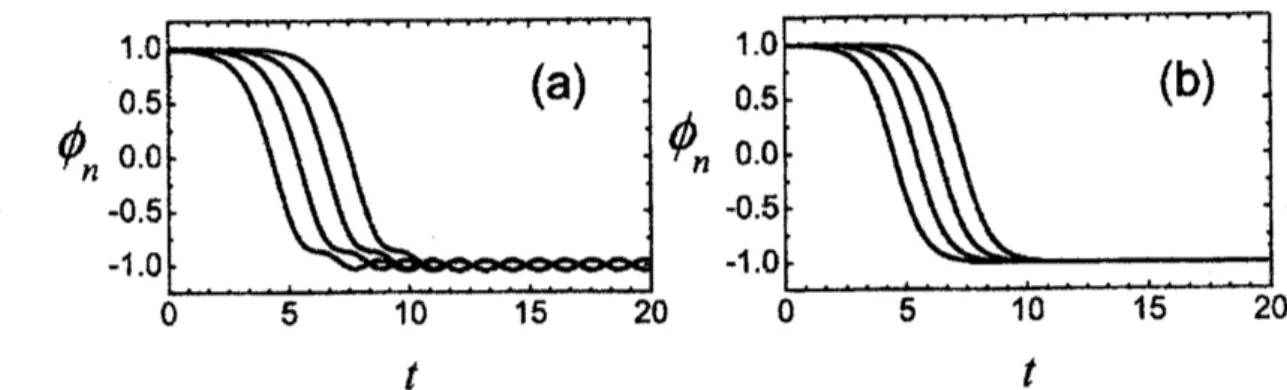
(a)

(b)

(C) 2.0 1.5 _.,, $\ldots$

..

$\cdot$ IIes 1.0 $\ldots\ldots\ldots\ldots..,\ldots\ldots\ldots\ldots.$

.

$\ldots\ldots\ldots\prime\prime\ldots\ldots.’\ldots\ldots\ldots$

.

$\cdots\ldots\ldots...$

.

$aJ$ $.\cdot\cdot\cdot\cdot\cdot\cdot\cdot\cdot\cdot$

.

0.5

_.,

$\cdot$

.

$\cdot$

.

$\cdot\dot{.}$

..

$\cdot$ 0.0 $\ldots\ldots$ $\ldots\ldots\ldots,\ldots..\sim$ $\ldots\ldots\ldots\ldots..’\cdots\cdots\cdots\cdots\cdot$

.

$.\cdot...$

.

.,

$\cdot$

.

$\cdot$

.

$\ldots\ldots..\cdot.\cdot$ .,,$\ldots$

..

$\ldots\ldots\ldots\prime\prime\ldots\ldots.’\ldots\ldots\ldots$

.

...,...,

.

$\ldots$, $\ldots\ldots\ldots...$

.

$.\dot{.}$ $\ldots\ldots\ldots,\ldots..\sim$ 0.5 1.5 2.0 0.5 1.0 1.5 2.0 0.5 1.0 t.5 2.0 $h$ $h$ $h$

$l$ $[\mathrm{x}70^{5}]$ $\mathrm{f}$ $[\mathrm{x}10^{5}]$ $t$ $\{\mathrm{x}10^{5}]$

Fig. 1. Upper panels: boundaries ofthe linear spectrum ofthe

vacuum

(solid lines) and

kinkinternal mode frequencies (dots)

as

functions of the lattice spacing $h$

.

Lower panels:

time evolution of kink velocity for different initial velocities and $h=0.7$ . The results

are

shown for (a) classical $\psi^{4}$ model, Eq. (34), (b) $\mathrm{P}\mathrm{N}\mathrm{p}$-ffee model conserving

energy,

Eq.

We analyze the kink internal modes (i.e., internal degrees of ffeedom [9]) for these

three models. First,

we

determine the kink-like

heteroclinic

solution by

means

of

relaxationaldynamics. Then,thelinearized equations

are

usedin

a

lattice of $N=200$ sites

to obtain $N$

eigenfrequencies

and the corresponding eigenmodes. We

are

particularly

interested in the eigenfrequencies which lie outside the linear vibration band of

vacuum

solutionandthus

are

associatedwiththekinkinternal modes. It isworthwhiletonotice that the eigenproblem for models conserving energy, Eq. (32) and Eq. (34), has

a

symmetric Hessian matrix while the non-self-adjoint problem for the momentum-conserving model Eq. (33) results in

a

non-symmetricmatrix.

The top panels ofFig. 1 present theboundaries of the linear vibration spectrum of the

vacuum

(solidlines) and the kink internal modes (dots)

as

the functions oflattice spacing

$h$ for(a) theclassical $\phi^{4}$ modelof Eq. (34), (b)the$\mathrm{P}\mathrm{N}\mathrm{p}$-freemodelofEq. (33)conserving

energy, and (c)the$\mathrm{P}\mathrm{N}\mathrm{p}$-free model ofEq. (32) conserving momentum. In

$\mathrm{P}\mathrm{N}\mathrm{p}$-ffee models

kinks possess

a

zero

ffequency, Goldstone translational mode similarly to the continuum

$\phi^{4}$ kink. Hence, the static kink

can

be centered anywhere

on

the lattice. The results

presented in Fig. 1

are

for thekinksituated exactly betweentwo lattice sites. Thisposition

is the stable position for the classical $\phi^{4}$ discrete kink [9]. Since all three discretemodels

share the

same

continuum $(\phi^{4})$ limit, their spectra

are

very close for small $h(<0.5)$

.

We

found that the model Eq. (32)

may

have kink intem al modes lying above the spectrum of

vacuum, e.g., for $\alpha=1/2$_, $\beta=0$, $\gamma=1/4$, and $\mathit{5}=0$

.

Suchmodes

are

short-wavelength

ones, with large amplitudes (energies) and they do not radiate because ofthe absence of

couplingtothe linearphonon spectrum.

$t$ $t$

Fig. 2. Trajectories particles (a) inthe model of Eq. (32) with $h=0.7$ when the kink

moves

with

a

steady velocity $v*$ (see Fig. 1(c), bottompanel)and(b) forthe

continuum

$\phi^{4}$

kink.

Perhaps

more

interesting

are

the implications ofsuchdiscretizations

on

themobility of

kinks. In the $\mathrm{P}\mathrm{N}\mathrm{p}$-ffee models, Eq. (32) and Eq. (33), the kink

was

launched using

a

perturbation along the Goldstone mode to provide the initial kick. In the classical model

Eq. (34) for this

purpose we

employed the imaginary frequency(real eigenvalue) unstable

eigenmode for

a

kink initialized at the unstable position (a site-centeredkink). In all

cases

the amplitude ofthe mode is relatedtothe initialvelocity of thekink. Jnthe bottom panels

ofFig. 1

we

present the time evolution ofthe kink velocity for different initial velocities

the classical $\phi^{4}$ model presented in (a) is much smaller than in the

$\mathrm{P}\mathrm{N}\mathrm{p}$-fiee models, (b)

and (c). Furthermore,

a

very interesting effectofkink

_{selfacceleration}

can

be observedin

panel (c). Here there exists

a

selected kink velocity $v=*$

0.637

_{and kinks launched with}

$v>v*$_{, in a very short time (cannotbe}

_seen

_{in the scaleof the figure) adjusttheir velocities}

to $v*$

.

Moresurprisingly, the velocity adjustment is observed

even

forkinks launched with

$v<v*.$ _{In the steady-state regime, when the kink}

_moves

_with $v=v*$_{, it excites (in its tail)}

the short-wave oscillatory mode

even

though in ffont of the kink the

vacuum

is not perturbed.

These results generate the question of where the energy for the self-acceleration and

vacuum

excitation

comes

fiiom. InFig. $2(\mathrm{a})$

we

show the trajectories offour neighboring

particles when

a

kinkmoving with $v=v*$ _{(see Fig. 1(c), bottom panel)}

moves

_{through. For}

comparison,in (b)thetrajectories forthe classical $\phi^{4}$ kink, _{$\phi_{\eta}(t)=\tanh[\rho(nh-vt)]$}, where

$p=1/\sqrt{2-2v^{2}}$_,

are

_{shown. In both}

cases

_{the trajectories}

_are

_{identical and shifted with}

respectto eachother by $t=h/v$_{,butin(b)they}

_are

_{the oddffinctions withrespectthe point}

$\phi_{n}=0$ while in(a) they

are

not. The workdone bythebackgroundforces,Eq. (5), to move

the $n$thparticlefrom

one

energy

well to anotheris

$W_{n}=- \int_{\mathrm{r}}^{\infty}\dot{m}B(l,m,r)dt$ . (35)

For the $\phi^{4}$ model Eq. (32) with _{$\beta=\gamma=\delta=0$}, the nonlinear part of $B(l,m,r)$ reduces

to $\mathrm{B}(\mathrm{I},\mathrm{m},\mathrm{r})=(1/2)m^{2}(l+r)$. It is straightforward to demonstrate that _{$W_{n}=0$} for the

classical $\phi^{4}$ kink. However, if

a

termbreaking oddsymmetry, e.g., ecosh-1$[\theta(nh-vt)]$, is

added to the kink, the work becomes nonzero,

$W_{n}=(\pi/2)e(e^{2}+1)[\cosh(ph)-1]^{3}/\sinh^{4}(ph)$_, where

we

set for simplicity $\theta=\rho$.

Numerically

we

found that $W_{n}$

can

be positive

or

negative depending

on

$\rho$,

$\theta$ and thekink

velocity, $v$

.

This simple analysis qualitatively explains the kink self-acceleration

or

decelerationand the

vacuum

excitation. The

energy

forthis

comes

fromthebreaking of the

odd symmetry of particle trajectories, which is possible in the case of path-dependent background forces. It is, thus, very interesting to highlight the distinctions between the

regular discrete models, the $\mathrm{P}\mathrm{N}\mathrm{p}$-free, energy conserving discrete models, and the

PNp-free, momentumconservingdiscrete models. The first

ones

lead to rapid dissipation of the

wave’skinetic

energy

due tothe PNbarrier. The secondrender the dissipation far slower in

time. Finallythe third may

even

sustainself-accelerating

waves

and lockingto

a

particular

speed due tothe non-potential nature of the relevantmodel,

8. Discussion and conclusions

A sufficient condition toobtain

a

discrete Klein-Gordonmodelwith static kinks ffee of

Peierls-Nabarro potential

was

given (Sec. 4). The$\mathrm{P}\mathrm{N}\mathrm{p}$-freemodels derived

so

far [1-3]

can

be extracted ffom this sufficientcondition

as

particular

cases.

-A number of characteristic similarities and differences between energy- and momentum-conserving $\mathrm{P}\mathrm{N}\mathrm{p}$-free discrete models

were

highlighted. The momentum

conserving Klein-Gordon system with non-potential background forces discussed here

sense

that the viscosity and external forces

are

not explicitly introduced. This makes the dynamics of the system peculiar, for example,

as

it

was

demonstrated, the existence, the intensity, andthe sign of

energy

exchange withthe surroundings depends

on

the symmetry

and othercharacteristicsof the motion.

It would be interesting to investigate if the sufficient condition of having

no

PNp

formulated in Sec. 4

can

be used to construct models conserving quantities other than

energyandmomentum.

Further investigation of the intriguing dynamicproperties ofsuch non-potential models is important, given the relevance ofpath-dependent forces invarious applications such as,

e.g., aerodynamic and hydrodynamic forces, the forces induced in

automatic

control

systemsandothers. Suchstudies

are

in

progress

and will be reported in futurepublications.

References

1. J. M. Speight and R. S. Ward, Nonlinearity 7, 475 (1994); J. M. Speight, Nonlinearity

10,

1615

(1997); J. M. Speight,Nonlinearity 12,

1373

(1999).

2. P. G. Kevrekidis,PhysicaD183,

68

(2003).

3. S. V. Dmitriev, P. G.Kevrekidis,N. Yoshikawa (submittedforpublication).

4. E. B. Bogomol’nyi,J. Nucl. Phys. 24,

449

(1976).

5. G. Parisi, Statistical FieldTheory, Addison-Wesley(NewYork, 1988).

6. R. K. Dodd, J. C. Eilbeck, J. D. Gibbon, and H. C. Morris, Solitons and Nonlinear

Wave Equations, Academic Press(London, 1982).

7. P. Anninos, S. Oliveira,and R. A. Matzner,Phys. Rev. D44, 1147 (1991).

8. T. I. Belova andA. E. Kudryavtsev, Phys. Uspekhi40,

359

(1997).

9. O. M. Braun, Yu. S. Kivshar, and M. Peyrard, Phys. Rev. E56,

6050

(1997); Yu. S. Kivshar et al., Phys. Rev. Lett. 80,

5032

(1998); P. G. Kevrekidis and C. K. R. T.