Uniform stability and attractivity for linear systems with periodic coefficients (New Developments of Functional Equations in Mathematical Analysis)

(1)

Uniform stability and

attractivity

for linear

systems

with periodic coefficients

杉江実郎 (Jitsuro Sugie)

DepartmentofMathematics andComputer Science,Shimane University

1

Introduction

Inthispaper,

we

considerthe linearsystem

$x’=A(t)x=(\begin{array}{ll}-r(t) p(t)-p(t) -q(t)\end{array})x$, (1)

where theprimedenotes$d/dt$; the coefficients$p(t),$$q(t)$ and$r(t)$

are

continuous for$t\geq 0$,and $p(t)$ is

a

periodicfimction with period$\omega>0$

.

System(1) has the

zero

solution$x(t)\equiv 0\in \mathbb{R}^{2}$

.

We say thatthe

zero

solution of(1) isattractive ifevery solution$x(t)$ of(1)tends to $0$

as

time

$t$ increases.

If$q(t)$ and$r(t)$

are

alsoperiodicfimctions with period$\omega$, Floquet’stheorem is available. Let

$\Phi(t)$ bethefimdamentalmatrixof(1)with $\Phi(0)=E$, the$2\cross 2$ identity matrix. Then $\Phi(\omega)$ is

called themonodromy matrixof(l). Let$\mu_{1}$ and$\mu_{2}$bethe eigenvaluesofthemonodromymatrix

$\Phi(\omega)$

.

The eigenvalues $\mu_{1}$ and $\mu_{2}$

are

often called the Floquet multipliers of(1). By Abel’s formula,

$\det\Phi(\omega)=\det\Phi(0)\exp(-\int_{0}^{\omega}(q(s)+r(s))ds)=\exp(-\int_{0}^{\omega}(q(s)+r(s))ds)$.

Thus, theFloquet multipliers$\mu_{1}$ and$\mu_{2}$

are

therootsofthe equation

$\mu^{2}-tr\Phi(\omega)\mu+\exp(-\int_{0}^{\omega}(q(s)+r(s))ds)=0$.

It is well-known thatthe

zero

solution of(1) is attractive if and only if the Floquet multipliers

$\mu_{1}$ and$\mu_{2}$ havemagnitudes strictly less than 1. Hence, in the

case

where$p(t),$ $q(t)$ and$r(t)$

are

periodic,necessary and sufficient conditions for the

zero

solution of(1)to beattractive

are

that

$| tr\Phi(\omega)|<1+\exp(-\int_{0}^{\omega}(q(s)+r(s))ds)$

and

$\exp(-\int_{0}^{\omega}(q(s)+r(s))ds)<1$.

(2)

Although the above conditions

are necessary

and sufficient for the

zero

solution of(1) to be attractive, it is difficult to

estimate

the absolute value ofthe trace of $\Phi(\omega)$, because it is

impossible to find

a

hndamental matrix of(1) in general. Of course, Floquet’s theorem is

useless when$q(t)$

or

$r(t)$ is notperiodic. Then, withoutknowledge of

a

ffindamental matrix _of

(1),

can we

_{decide whether the}

_zero

_solution_is _{attractive? What kind of condition}

_on

$A(t)$ will

guaranteetheattractivity ofthe

zero

solution of(1)?

2

The

main

theorem

Togive

an answer

tothe abovequestion,

we

prepare

some

notations. Let

$R(t)= \int_{0}^{t}r(s)ds$ and _{$\psi(t)=2(q(t)-r(t))$}

for$t\geq 0$anddenote apositive partand anegative partof$\psi(t)$ by

$\psi_{+}(t)=\max\{0, \psi(t)\}$ and $\psi_{-}(t)=\max\{0, -\psi(t)\}$,

respectively. Note that$\psi(t)=\psi_{+}(t)-\psi_{-}(t)$ and $|\psi(t)|=\psi_{+}(t)+\psi_{-}(t)$

.

We introduce

an

important concept here. Anonnegative ffinction$\phi(t)$ is said to be weakly

integrallypositiveif

$l\phi(t)dt=\infty$

for every set $I= \bigcup_{n=1}^{\infty}[\tau_{n}, \sigma_{n}]$ such that _{$\tau_{n}+\delta<\sigma_{n}<\tau_{n+1}<\sigma_{n}+\Delta$}for

some

_$\delta>0$ and

$\triangle>0$

.

For example, _$1/(1+t)$ and

$\sin^{2}t/(1+t)$ areweakly integrallypositiveRnctions _(see

[6,7, 13-15]$)$.

Our mainresultis stated

as

follows:

Theorem 1. Suppose that $q(t)$ and$R(t)$

are

boundedfor

$t\geq 0$. Supposealsothat

(i) $\psi_{+}(t)$ isweakly integrally positive;

(ii) $\int_{0}^{\infty}\psi_{-}(t)dt<\infty$.

Then thezerosolution

_of

(1) is attractive.

Toprove Theorem 1, weneedsomelemmas. We presentthe lemmas without theproofs.

Lemma 2. Suppose that assumption (ii) in Theorem 1 holds. Let $v(t)$ be nonnegative and

continuously

_{differentiable}

on $[t_{0}, \infty)$

for

some

_{$t_{0}>0$}.

If

(3)

then$v’(t)$ isabsolutelyintegrable,and

therefore

$v(t)$ hasanonnegative limitingvalue.

Lemma3. Supposethat$R(t)$ is

boundedfor

$t\geq 0$

.

If

assumption(ii)in Theorem 1 holds,then

all solutions

_of

(1)

are

unifomly stableanduniformlybounded.

Recall that$p(t)$ is

a

periodic fimctionwithperiod$\omega>0$

.

Let

$\overline{p}=\max_{t\in[0,\omega]}p(t)$ and $\underline{p}=\min_{t\in[0,\omega]}p(t)$

.

Taking$\overline{p}\geq\underline{p}$intoaccount,

we

see

that if$\overline{p}+\underline{p}\geq 0$, then$\overline{p}>0$; if$\overline{p}+\underline{p}<0$,then$\underline{p}<0$

.

Since

$p(t)$ is continuous for$t\geq 0$,

we see

that$p(t)$hasthe following property(we

omit

theproof).

Lemma 4. Let$m$ be anyinteger.

If

$\underline{p}+\overline{p}\geq 0$, then there existnumbers$a$and$b$with$0\leq a<$

$b\leq\omega$suchthat

$p(t) \geq\frac{1}{2}\overline{p}>0$

for

_{$m\omega+a\leq t\leq m\omega+b$}

.

If

$\underline{p}+\overline{p}<0$, then there exist numbers $a$and$b$with$0\leq a<b\leq\omega$such that $p(t) \leq\frac{1}{2}\underline{p}<0$ for _{$m\omega+a\leq t\leq m\omega+b$}

.

3

Proof of

the

main

theorem

We

are now

readyto proveTheorem 1.

ProofofTheorem1. Let$x(t;t_{0}, x_{0})$be

a

solutionof(l)passingthrough$(t_{0}, x_{0})\in[0, \infty)\cross \mathbb{R}^{2}$

.

It follows ffom Lemma 3 that for any $\alpha>0$, there exists

a

$\beta(\alpha)>0$ such that $t_{0}\geq 0$ and

$\Vert x_{0}\Vert<\alpha$imply that

$\Vert x(t;t_{0}, x_{0})\Vert<\beta$ for $t\geq t_{0}$

.

(3)

Forthesakeofbrevity,

we

write $(x(t), y(t))=x(t;t_{0}, x_{0})$ and

$v(t)=V(t, x(t), y(t))$ .

Then,

we

have

$v(t)= \frac{1}{2}e^{2R(t)}(x^{2}(t)+y^{2}(t))$ (4)

and

$v^{f}(t)=-(q(t)-r(t))e^{2R(t)}y^{2}(t)\leq\psi_{-}(t)v(t)$ (5)

for $t\geq t_{0}$

.

Hence, ffom Lemma 2,

we

see

that$v(t)$ has

a

limiting value$v_{0}\geq 0$

.

If$v_{0}=0$,then

by (4) the solution $(x(t), y(t))$ tends to $0$

as

$tarrow\infty$

.

This completes the proof. Thus, we need

consider only the

case

inwhich $v_{0}>0$. Wewill show that this

case

doesnot

occur.

Becauseof(3),

we

see

that $|y(t)|$ is bounded for$t\geq t_{0}$. Hence, $|y(t)|$ has

an

inferior limit

and

a

superior limit. First,

we

will show that theinferior limit of$|y(t)|$ is zero, and

we

will then

(4)

Suppose that $hm\inf_{tarrow\infty}|y(t)|>0$

.

Then, there exist

a

$\gamma>0$ and

a

$T_{1}\geq t_{0}$ such that

$|y(t)|>\gamma$for$t\geq T_{1}$

.

Itfollows from(5) and Lemma 2 that

$\infty>\int_{t_{0}}^{\infty}|v’(s)|ds=\frac{1}{2}\int_{t_{0}}^{\infty}|\psi(s)|e^{2R(s)}y^{2}(s)ds$

$\geq\frac{1}{2}\gamma^{2}\int_{T_{1}}^{\infty}\psi_{+}(s)e^{2R(s)}ds\geq\frac{1}{2}\gamma^{2}e^{-2L}\int_{T_{1}}^{\infty}\psi_{+}(s)ds$,

where $L$ isthe number givenintheproofof Lemma3. This contradicts assumption

(i). Thus,

we see

that$\lim\inf_{tarrow\infty}|y(t)|=0$

.

Suppose that $\lim\sup_{tarrow\infty}|y(t)|>0$

.

Let $\nu=\lim\sup_{tarrow\infty}|y(t)|$

.

Since $q(t)$ is bounded,

we

can

find

a

$\overline{q}>0$ such that

$|q(t)|\leq\overline{q}$ for $t\geq 0$

.

(6)

Since$v(t)$ tends to

a

positive value$v_{0}$

as

$tarrow\infty$,there exists

a

$T_{2}\geq t_{0}$ suchthat

$0< \frac{1}{2}v_{0}<v(t)<\frac{3}{2}v_{0}$ for $t\geq T_{2}$

.

(7)

Let$\epsilon$be

so

smallthat

$0< \epsilon<\min\{\frac{1}{2}\nu,$ $\sqrt{\frac{\overline{p}^{2}e^{-2L}v_{0}}{4(\overline{q}+2/(b-a))^{2}+\overline{p}^{2}}},$ $\sqrt{\frac{\underline{p}^{2}e^{-2L}v_{0}}{4(\overline{q}+2/(b-a))^{2}+\underline{p}^{2}}}\}$, (8)

where $a$and $b$

are

the numbers given in Lemma4. Then, since

$\lim\inf_{tarrow\infty}|y(t)|=0$,

we

can

selecttwointervals $[\tau_{n}, \sigma_{n}]$ and $[t_{n}, s_{n}]$with $[t_{n}, s_{n}]\subset[\tau_{n}, \sigma_{n}],$$T_{2}<\tau_{n}$and$\tau_{n}arrow\infty$

as

$narrow\infty$

suchthat $|y(\tau_{n})|=|y(\sigma_{n})|=\epsilon,$ _{$|y(t_{n})|=\nu/2,$ $|y(s_{n})|=3\nu/4$} and

$|y(t)|\geq\epsilon$ for $\tau_{n}<t<\sigma_{n}$, (9)

$|y(t)|\leq\epsilon$ for $\sigma_{n}<t<\tau_{n+1}$, (10)

$\frac{1}{2}\nu<|y(t)|<\frac{3}{4}\nu$ for _{$t_{n}<t<s_{n}$}. ₍₁₁₎

By(4), (7) and(10),

_we

have

$|x(t)|=\sqrt{2e^{-2R(t)}v(t)-y^{2}(t)}\geq\sqrt{e^{-2L}v_{0}-\epsilon^{2}}$ ₍₁₂₎

for$\sigma_{n}\leq t\leq\tau_{n+1}$.

Claim. The sequences$\{\tau_{n}\}$ and $\{\sigma_{n}\}$ satisfy _{$\tau_{n+1}-\sigma_{n}\leq 2\omega$} forany integer _$n$

.

Suppose thatthere exists

an

$n_{0}\in N$such that $\tau_{no+1}-\sigma_{n0}>2\omega$

.

We

can

choose

an

$m\in N$

such that$(m-1)\omega<\sigma_{n_{0}}\leq m\omega$. Hence,

we

have

$\tau_{n_{0}+1}>\sigma_{n_{0}}+2\omega>(m-1)\omega+2\omega=(m+1)\omega$,

and therefore $[rr\iota\omega, (m+1)\omega]\subset[\sigma_{n_{0}}, \tau_{n_{0}+1}]$. There

are

two

cases

to consider: (a)

$\overline{p}+\underline{p}\geq 0$

(5)

$[m\omega, (m+1)\omega]$

.

Hence, using the second equation in system (1) with (6), (10) and (12),

we

have

$|y’(t)| \geq|p(t)||x(t)|-|q(t)||y(t)|\geq\frac{1}{2}\overline{p}\sqrt{e^{-2L}v_{0}-\epsilon^{2}}-\overline{q}\epsilon$ (13)

for $a+m\omega<t<b+m\omega$

.

_Itfollows $\theta om(8)$ that

$\frac{1}{2}\overline{p}\sqrt{e^{-2L}v_{0}-\epsilon^{2}}-\overline{q}\epsilon>\frac{2}{b-a}\epsilon$

.

(14)

From (10) and(13),

we

can

estimate that

$2 \epsilon\geq|y(b+m\omega)|+|y(a+m\omega)|\geq|\int_{a+\pi\omega}^{b+m\omega}y^{f}(s)ds|$

$= \int_{a+\pi w}^{b+\pi\omega}|y’(s)|ds\geq(b-a)(\frac{1}{2}\overline{p}\sqrt{e^{-2L}v_{0}-\epsilon^{2}}-\overline{q}\epsilon)$

.

This contradicts (14). In

case

(b), by Lemma 4,$p(t)\leq\underline{p}/2<0$ for $t\in[a+m\omega, b+m\omega]\subset$

$[m\omega, (m+1)\omega]$

.

Hence, combiningthis with(6), (10) and(12),

we

obtain

$|y^{f}(t)| \geq|p(t)||x(t)|-|q(t)||y(t)|\geq-\frac{1}{2}\underline{p}\sqrt{e^{-2L}v_{0}-\epsilon^{2}}-\overline{q}\epsilon$ (15)

for$a+m\omega<t<b+m\omega$

.

_It_follows _Rom₍₈₎ _that

$- \frac{1}{2}\underline{p}\sqrt{e^{-2L}v_{0}-\epsilon^{2}}-\overline{q}\epsilon>\frac{2}{b-a}\epsilon$

.

(16)

From (10) and(15),

we

can

estimate that

$2 \epsilon\geq|y(b+m\omega)|+|y(a+m\omega)|\geq|\int_{a+\pi w}^{b+m\omega}y’(s)ds|$

$= \int_{a+mtd}^{b+\pi\omega}|y^{f}(s)|ds\geq(b-a)(-\frac{1}{2}\underline{p}\sqrt{e^{-2L}v_{0}-\epsilon^{2}}-\overline{q}\epsilon)$.

This contradicts (16). Thus,the claim isproved.

Let $I= \bigcup_{n=1}^{\infty}[\tau_{n}, \sigma_{n}]$

.

Then, by

means

ofLemma2 with(5) and (9),

we

get

$\infty>\int_{t_{0}}^{\infty}|v’(s)|ds=\frac{1}{2}\int_{t_{0}}^{\infty}|\psi(s)|e^{2R(s)}y^{2}(s)ds$

$\geq\frac{1}{2}e^{-2L}\int_{t_{0}}^{\infty}\psi_{+}(s)y^{2}(s)ds\geq\frac{1}{2}\epsilon^{2}e^{-2L}\int_{I}\psi_{+}(s)ds$.

Hence, it follows from assumption (i) and the claim that $\lim\inf_{narrow\infty}(\sigma_{n}-\tau_{n})=0$

.

Since

$[t_{n}, s_{n}]\subset[\tau_{n}, \sigma_{n}]$,it follows that

(6)

By(4), (7)and (11),

we

have

$|x(t)|=\sqrt{2e^{-2R(t)}v(t)-y^{2}(t)}\leq\sqrt{3e^{2L}v_{0}-\frac{\nu^{2}}{4}}$

for$t_{n}\leq t\leq s_{n}$

.

Let$K= \max\{|\overline{p}|, |\underline{p}|\}$

.

Then,from (6)and(11),

we

see

that

$|y’(t)| \leq|p(t)||x(t)|+|q(t)||y(t)|<K\sqrt{3e^{2L}v_{0}-\frac{\nu^{2}}{4}}+\frac{3}{4}\overline{q}\nu$

for$t_{n}\leq t\leq s_{n}$

.

Letting $N=K\sqrt{3e^{2L}v_{0}-\nu^{2}}/4+3\overline{q}\nu/4$ and integrating this inequality ffom

$t_{n}$to _{$s_{n}$},we obtain

$\frac{1}{4}\nu=|y(s_{n})|-|y(t_{n})|\leq|y(s_{n})-y(t_{n})|$

$=| \int_{t_{n}}^{s_{\hslash}}y^{f}(s)ds|\leq\int_{t_{n}}^{s_{n}}|y’(s)|ds\leq N(s_{n}-t_{n})$

.

This contradicts (17). We therefore concludethat$\lim\sup_{tarrow\infty}|y(t)|=\nu=0$

.

In

summary,

$y(t)$ tends to

zero as

$tarrow\infty$

.

Hence,there exists

a

$T_{3}\geq T_{2}$ such that

$|y(t)|<\epsilon$ for $t\geq T_{3}$. (18)

Let $l$ be

an

integer satisfying

$l\omega>T_{3}$

.

Using (18) instead of (10) and following the

same

process

as

in theproofoftheclaim,

we see

that if$\overline{p}+\underline{p}\geq 0$, then

$2 \epsilon\geq|y(b+l\omega)|+|y(a+l\omega)|\geq|\int_{a+l\omega}^{b+l\omega}y’(s)ds|$

$= \int_{a+l\omega}^{b+l\omega}|y’(s)|ds\geq(b-a)(\frac{1}{2}\overline{p}\sqrt{e^{-2L}v_{0}-\epsilon^{2}}-\overline{q}\epsilon)>2\epsilon$,

which isacontradiction; if$\overline{p}+\underline{p}<0$, then

$2 \epsilon\geq|y(b+l\omega)|+|y(a+l\omega)|\geq|\int_{a+l\omega}^{b+l\omega}y’(s)ds|$

$= \int_{a+l\omega}^{b+l\omega}|y’(s)|ds\geq(b-a)(-\frac{1}{2}\underline{p}\sqrt{e^{-2L}v_{0}-\epsilon^{2}}-\overline{q}\epsilon)>2\epsilon$,

which is again

a

contradiction. Thus,the

case

of$v_{0}>0$cannothappen.

The proof of Theorem 1 is thus complete. $\square$

4 Examples

Weillustrate

our

mainresult withsimpleexamples inwhich$p(t),$$q(t)$and$r(t)$

are

periodic. Itis

well-knownthat ifthe

zero

solutionof

a

linear periodicsystemisattractive,then itisuniformly

(7)

Example 1. Let $\lambda>0$

.

Considersystem(1)with

$p(t)=\cos t$, $q(t)= \frac{\lambda}{2-nt}$ and $r(t)=0$

.

(19)

Thenthe

zero

solution

is attractive.

Since $\lambda/3\leq q(t)\leq\lambda$ and $R(t)\equiv 0$, it is clearthat $q(t)$ and $R(t)$

are

bounded for $t\geq 0$

.

Also, assumptions(i)and(ii)

are

satisfied. Infact,

we

have

$\psi(t)=2(q(t)-r(t))=\frac{2\lambda}{2-\sin t}$,

and therefore

$\psi_{+}(t)=\frac{2\lambda}{2-\sin t}$ and $\psi_{-}(t)=0$

for$t\geq 0$

.

Hence,$\psi_{+}(t)$ isweakly integrallypositive and

$\int_{0}^{\infty}\psi_{-}(t)dt=0$

.

Thus,by

means

ofTheorem 1,

_we

conclude that the

zero

solutionis attractive.

Figure l(a) shows

a

positive orbit of(1) with (19) and $\lambda=0.1$

.

The starting point $x_{O}$ is

$(-1,0)$ and the initialtime$t_{0}$ is$0$

.

Thepositive orbit

moves

aroundthe origin$0$ in

a

clockwise

and

a

counter-clockwise direction altemately,because$p(t)$ changes its sign. The positive orbit

approaches the origin$0$

as

it

goes

upand down.

(a) (b)

Figure 1: (a)Apositive orbit of(1) with (20); (b)

a

positiveorbit of(1) with (21)

Example2. Let $\lambda\geq 1$

.

Considersystem (1)with

$p(t)=\cos\lambda t$, $q(t)=\cos^{2}t+\sin t$ _and $r(t)=\sin$_t. ₍₂₀₎

(8)

It

is

easy

to check that$q(t)$ and $R(t)$

are

bounded for$t\geq 0$and that assumptions(i) and(ii)

are

satisfied. We omit the details.

InFigure 1(b),

we

show

a

positiveorbit of(1)with(20)and $\lambda=4$

.

Thepositive orbitstarts

Rom thepoint $(-1,0)$ atthe initialtime$0$

.

The positiveorbitgoestotherightand then

goes

to

theleft, and itrepeatssuch

a

movementregularly. Although the positiveorbitdisplaysintricate

behavior,itapproaches theorigin $0$ultimately.

InExamples 1 and2, all coefficients of(1)

are

periodic hncbons withperiod $2\pi$

.

However,

we

camot find the monodromy matrix $\Phi(2\pi)$

.

It is particularly hard to estimate the absolute

value of the trace of$\Phi(2\pi)$. Forthis reason,

we

cannot apply Floquet’s theoremtoExamples 1

and2 directly. Theorem 1 hasthe advantageofbeing applicable to

cases

wherethemonodromy

matrixof(1)camotbe found and

cases

where$q(t)$

or

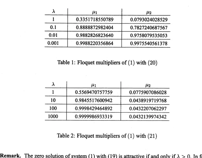
$r(t)$ isnotperiodic.

Fortunately, in Examples 1 and 2 the Floquet multipliers $\mu_{1}$ and $\mu_{2}$

can

be calculatedby

a

numerical scheme. As shown in Tables 1 and 2, $|\mu_{1}|<1$ and $|\mu_{2}|<1$

.

Hence,

we

see

thatthe

zero

solution of(1) isattractive.

Table 1: Floquet multipliers of(1) with (20)

Table2: Floquet multipliers of(1) with (21)

Remark. The

zero

solution ofsystem(1) with (19) is attractive ifandonly if$\lambda>0$

.

Infact,if

$\lambda\leq 0$, then

$\exp(-\int_{0}^{\omega}(q(s)+r(s))ds)=\exp(-\int_{0}^{\omega}\frac{\lambda}{2-\sin s}ds)\geq 1$.

(9)

References

[1] A.BacciottiandL. Rosier, LiapunovFunctions and StabilityinControl Theory, 2nded.,

Spninger-Verlag, Berlin-Heidelberg-NewYork,2005.

[2] F. Brauer andJ. Nohel, The Qualitative Theory

_of

Ordinary

_Differential

Equations, W. A.

Ben-jamin,NewYorkandAmsterdam, 1969;(revised)Dover,NewYork, 1989.

[3] J. Cronin,

_Differential

Equations: Introductionand Qualitative Theory, 2nded., Monographsand Textbooks in Pure andAppliedMathematics 180,Marcel Dekker,New York-Basel-Hong Kong,

1994.

[4] A. Halanay,

_Differential

Equations: Stability,Oscillations,fime Lags,AcademicPress,NewYork–

London, 1966.

[5] J. K. Hale, Odinary

_Differential

Equations,Wiley-Interscience, New York-London-Sydney, 1969;

(revised)Knieger,Malabar, 1980.

[6] L. Hatvani, On the asymptoticstability bynondecrescent Ljapunovfunction, NonlinearAnal., 8

(1984), 67-77.

[7] L. Hatvani, On the asymptotic stability

_for

a two-dimensional linearnonautonomous

_differential

system,NonlinearAnal., 25(1995),991-1002.

[8] D. W.Jordan and P.Smith,Nonlinear Ordinary

_Differential

Equations: Anintmductionto

Dynam-ical Systems, 3rded., OxfordTextsinAppliedand Engineering Mathematics2,OxfordUniversity

Press,Oxford, 1999.

[9] J. P. LaSalle and S. Lefschetz, Stability by LiapunovS DirectMethodwith Applications,

Mathe-matics in Scienceand Engineering 4, AcademicPress,NewYork-London, 1961.

[10] D. R.Merkin,Introductiontothe Theory

_of

Stability, TextsinAppliedMathematics24,

Springer-Verlag, New York-Berlin-Heidelberg, 1997.

[11] A. N. Michel, L. Hou and D. Liu, Stobility Dynamical Systems: Continuous, Discontinuous, and

DiscreteSystems, Birkh\"auser,Boston-Basel-Berlin, 2008.

[12] N. Rouche, P.Habets and M. Laloy, Stability Theoyby Liapunov’sDirectMethod,Applied

Math-ematicalSciences22,Springer-Verlag, New York-Heidelberg-Berlin, 1977.

[13] J. Sugie, Convergence

_of

solutions

_of

time-varying linearsystem with integrableforcing term,

Bull. Austral. Math. Soc.,78 (2008), 445-462.

[14] J. Sugie,

_Influence

_of

anti-diagonals on the asymptotic stability

_for

linear

_differential

systems, Monatsh. Math., 157(2009), 163-176.

[15] J. Sugie and Y. Ogami, Asymptotic stability

_for

three-dimensional linear

_differential

systems with

time-varyingcoefficients,toappear inQuart. Appl. Math.

[16] F. Verhulst,Nonlinear

_Differential

EquationsandDynamical Systems, Springer-Verlag, New

York-Berlin-Heidelberg, 1990.

[17] T. Yoshizawa, Noteontheboundedness and theultimateboundedness

_ofsolutions

_of

$x’=F(t,$x),

(10)

[18] T. Yoshizawa,Stability Theory by Liapunov’sSecondMethod,Math. Soc. Japan, Tokyo, 1966.

[19] T. Yoshizawa, Stability Theo,y and the Existence

_of

PeriodicSolutions andAlmostPeriodic