Optimal Testing/Maintenance Design in a Software Development Project (Development of the Dynamic Systems under Uncertainty)

72

Optimal

$\mathrm{T}\mathrm{e}\mathrm{s}\mathrm{t}\mathrm{i}\mathrm{n}\mathrm{g}/\mathrm{M}\mathrm{a}\mathrm{i}\mathrm{n}\mathrm{t}\mathrm{e}\mathrm{n}\mathrm{a}\mathrm{n}\mathrm{c}\mathrm{e}$

Design

in

a

Software

Development Project

林坂弘一郎, 土肥正

Koichiro Rinsaka and Tadashi

Dohi

Department

of

Information

Engineering,

Graduate

School

of Engineering,

Hiroshima

University, Japan

1

Introduction

It is important to determine the optimal time when softwaretesting should be stopped and when the

systemshouldbe deliveredto

a user or

amarket. This problem, called optimal

_software

releaseproblem, plays a central role for the success orfailure ofa software development project. Okumoto and Goel [1]

assumed thatthe numberofsoftware faults detected inthe testingphase is describedby

an

exponential

software reliability model based on a non-homogeneous Poisson process (NHPP) [2], and derived

an

optimal software release timewhich minimizes the total expected software cost. Koch and Kubat [3]

considered the similar problem for theother softwarereliabilitymodel by Jelinski and Moranda [4]. Bai

and Yun [5] calculated the optimal number of faults detected before the release under the Jelinski and

Moranda model. Many authors formulated the optimal software release problems based

on

different

model assumptions $\mathrm{a}\mathrm{n}\mathrm{d}/\mathrm{o}\mathrm{r}$several softwarereliability models $[6, 7]$.

It is difficult to detect and

remove

allfaultsremainingin

a

softwareduringthetesting phase, because

exhaustivetestingofallexecutable paths in

a

generalprogram isimpossible. Once the software is released

tousers, howeverthesoftwarefailures may

occur even

in the operational phase. It is

common

for software

developers to provide maintenance service during the period when they

are

still responsible for fixing

software faults causing failures. In order to carry out the maintenance in the operational phase, the

softwaredeveloper hasto keep

a

software maintenance team. At the

same

time, the management cost

in the operational phase should be reduced

as

much

as

possible, but the human

resources

should be utilized effectively. Although the problem which determinesthe maintenanceperiod is importantfrom

the practical point ofview, only

a

veryfew authors paid theirattention tothis problem.

Kimura et al. [8] considered the optimal software release problem in the

case

where the software

warranty period is a random variable. Pham and Zhang [9] developed

a

software cost model with both

warranty and risk. Theyfocused

on

theproblemfor determining when tostopthesoftwaretestingunder

a

warrantycontract. However,

it is

noted that the software developer has to design thewarrantycontract

itselfandoftenprovidesthe posteriorservice for

users

after softwarefailures. Dohi et $a/$

.

[10]formulated

the problem for determining the optimalsoftwarewarranty periodwhich minimizes the total expected

software cost under theassumption that the debugging process in the testing phase is described by

an

NHPP. Since the user’s operational environment is not always

same as

that assumed in the software

development phase, however, the above literature did not take account ofthe difference between two

different phases.

Several reliability assessment methods during the operational phase have been proposed by

some

authors $[11, 12]$

.

_{In this} paper,

we

develop

a

stochastic model for designing the optimal testing and

maintenanceperiods, where thedifferencebetween thesoftwaretesting environmentand the operational

environment

are

reflected. Based

on

the idea in Okamura et al. [12],

we

formulate the total expected

software cost incurred for the software developer, and derive analytically the optimal testing period

(release time) which

minimizes

the total expected software cost. Wecall the time length to complete

the operational

maintenance

after the release

a

plannedmaintenance limit, and alsoderive the optimal

planned

maintenance

limit which

minimizes

the total expected

software

cost. Throughout

numerical

examples,

we

calculate numerically the joint optimal policy combined by testing period and planned

maintenance limit. Finally, the paper is concluded with

some

remarks.

2

Model

Description

First,we make the followingassumptions

on

thesoftware fault-detection process:

73

(a) In each time when

a

software failure occurs, the software fault causing the failure is detected and

removed immediately.

(b) The number of initial faults contained in the software program, $N_{0}$, is given by the Poisson dis

tributedrandom variablewith

mean

$\omega$ $(>0)$

.

(c) The time to detect each software fault is independent and identically distributed nonnegative random variable with (absolutely continuous) probability distribution function $F(t)$ and density

function $f(t)$

.

Let $\{N(t), t\geq 0\}$ be the cumulative number of software faults detected up to time $t$. From the above

assumptions, the probability math function of$N(t)$ is given by

$\mathrm{P}\mathrm{r}\{N(t)=m\}=\frac{[\omega F(t)]^{m}e^{-\omega F(t)}}{m!}$ $m=0,1,2$,$\cdots$

.

(1)

Hence, the stochastic process $\{N(t), t\geq 0\}$ isequivalent to

an

NHPP with

mean

valuefunction$\omega F(t)$

,

where the

fault-detection rate

(debugging rate) per

unit

of

time

isgivenby

$r(t)= \frac{f(t)}{1-F(t)}$

.

(2)

Supposethat

a

software testing isstartedattime0and terminated at time$t_{0}(\geq 0)$

.

Thetimelength

ofsoftware lifecycle $t_{L}(>0)$ isknown in advance andis assumed to be sufficiently larger than$t_{0}$

.

More

precisely, thesoftware life cycle is measured from the time$t_{0}$

.

The software developer is responsible to

the maintenance service for all the software failures that mayoccurduring the software life cycle under

a maintenance contract. We suppose that the project manager decides to break up the maintenance

team at time$t_{0}+t_{W}(0\leq t_{W}\leq t_{L})$for reductionof the operational cost tokeep it, but

a

large amount

of debugging cost after the planned maintenance limit if the software failure occurs may be needed. Further,we define the following cost components;

$c_{0}(>0)$: cost to

remove

each fault in thetesting phase,

$c_{W}(>0)$: cost to

remove

each fault before the planned maintenance_limit, $cL$ $(>0)$: cost to

remove

each fault afterthe planned maintenance limit,

$k_{0}(>0)$: testingcost per unit oftime,

$kw$ $(>0)$: operationalcost to keepthe maintenance team per unitof time.

In the following section, we formulate the total expected software cost by introducing the above cost

factorsin testing andoperationalphases. We derive the optimalsoftwaretesting period

or

the optimal

planned maintenancelimit which minimizes the total expected software cost atthe endof the software life cycle. Then,

we

calculate the joint optimal policy combined by both testing period and planned

maintenance limit.

3

Total Expected Software

Cost

We

formulate

the totalexpected software cost which

can occur

in both testing and operational phases.

In theoperationalphase,

we

consider twocost factors;themaintenancecost due tothesoftware failure

and theoperationalcost tokeepthe maintenance team.

From Eq.(l), the probability math

function

of the number of software faults detected during the

testingphase isgiven by

$\mathrm{P}\mathrm{r}\{N(t_{0})=m\}=\frac{[\omega F(t_{0})]^{m}e^{-\omega F(t_{0})}}{m!}$

.

(3)

It should benoted thattheoperationalenvironment afterthe releasemay differ fromthe debugging

environment in thetesting phase. Thisdifference is similar to that between the accelerated life testing

environment and the normal operating

environment

for hardware products. Weintroduce the

74

andconsider that the timesinthe testing phaseand theoperationalphasehave a proportional

relation-ship. Namely, the time length $t$ in the operational phase correspondsto at in the testing phase. Under

the aboveassumption, $a=1$

means

theequivalence between the testing and operational

environments.

On the other hand, $a>1(a<1)\mathrm{i}$mplies that the operational

environment

is

severe

(looser) than the

testing environment. Okamura et al. (2001) applythis technique to model the operational phase of the software, and estimate the software reliability through an example inthe actual software development project. The probability math function ofthe number ofsoftware faults detected before the planned

maintenance limit is given by

$\mathrm{P}\mathrm{r}\{N(t_{0}+t_{W})-N(t_{0})= 72\}$$= \frac{\{\omega[F(t_{0}+at_{W})-F(t_{0})]\}^{m}}{m!}e^{-\omega[F\langle t_{0}+at_{W})-F(t_{0})]}$

.

(4)

Similarly, the fault-detectionprocessof thesoftwareafter the planned maintenance limit is expressed by

$\mathrm{P}\mathrm{r}\{N(t_{0}+t_{L})-N(t_{0}+t_{W})=m\}$

$=$ $\frac{\{\omega[F(t_{0}+at_{L})-F(t_{0}+at_{W})]\}^{m}}{m!}e^{-w}$[

$F(t_{0}+at\mathrm{D}-F(t0+\mathrm{a}\mathrm{t}\mathrm{w})$

(5)

FromEqs.(3), (4) and (5), the total expected software cost is given by

$\mathrm{C}(\mathrm{t}0, t_{W})$ $=$ $k_{0}t_{0}+$coU)F(to)$+k_{W}t_{W}+c_{W}\omega$[$F$($t_{0}+$atyy) -N(tO)

1$c_{L}\omega[F(t_{0}+at_{L})-F(t_{0}+atw)$

.

(6)

4

Determination of the Optimal Policies

In this section we derive the optimal testing period or the optimal planned maintenance limit which minimizes the total expectedsoftwarecost incurred to thesoftwaredeveloper at the end of software life cycle. Suppose that the time to detect each software fault obeys the exponential distribution [2] with

mean

$1/\lambda$ $(>0)$

.

Inthiscase, the total expected softwarecost in Eq.(6) becomes

$C(t_{0},t_{W})$ $=$ $\mathrm{k}\mathrm{o}\mathrm{t}0+c_{0}\omega(1-e^{-\lambda t_{0}})$ $+kwtw$

$+c_{W}\omega e^{-\lambda t_{0}}(1-e^{-\lambda at_{W}})+c_{L}\omega e^{-\lambda t_{\mathrm{O}}}(e^{-\lambda at_{W}}-e^{-\lambda at_{L}})$

.

(7)

Wemake thefollowing assumptions:

(A-I) $c_{L}>c_{W}>c_{0}$,

(A-II) $c_{W}(1-e^{-\lambda at_{L}})>c_{0}$,

(A-III) $c_{W}(1-e^{-\lambda at_{W}})+c_{L}(e^{-\lambda at_{W}}-e^{-\lambda at_{L}})>c_{0}$

.

Define

$Q(t_{W})=k_{0}+\omega\lambda[c_{0}-c_{W}(1-e^{-\lambda at_{W}})-c_{L}(e^{-\lambda at_{W}}-e^{-\lambda at_{L}})]$

.

(8)

Then the following result provides the optimal software testing policy which minimizes the total expected

software cost.

Theorem 1: When the

_{software fault-detection}

time distribution

_follows

the exponential distribution

with

mean

$1/\lambda$, under theassumptions (A-I) to (A-III), the optimal

software

testingperiod (release time)

which minimizes the total expected

_software

costis given

as

_follows:

(1)

_If

$Q(t_{W})<0,$ then there eists

a

finite

and unique optimal $sof$ tware testing period (release time) $t_{0}^{*}(>0)$, and its associated expected cost is given by

$C(t_{0}^{*},t_{W})$ $=$ $\mathrm{k}\mathrm{o}\mathrm{t}0+c_{0}\omega(1-e^{-\lambda t_{\mathrm{O}}^{*}}$

)

$1$kwtw

$+cw\omega e^{-\lambda}t$

;

_{$(1-e^{-\lambda at_{W}})+$}

$c_{L}$

$\mathrm{i}e^{-\lambda t_{\dot{0}}}$

(

$e^{-\lambda a}$t$W_{-e^{-\lambda at}}L$

)

\dagger (9)

(2)

_If

$Q(tw)\geq 0$

,

then the optimalpolicy is$t_{0}^{*}=0$ with

75

Proof: Forthe total expected cost in Eq.(7),we have

$5(0, t_{W})=kwtw$ $+c\iota V\omega$$(1-e^{-\lambda t_{W}})+c_{L}w$ $(e^{-\lambda at_{W}}-e^{-\lambda at_{L}})$ (11)

and

linl $\mathrm{C}$(tO$\mathrm{i}t_{W}$) $=+\mathrm{o}\mathrm{o}$. (12)

$t_{0}arrow+\infty$

Differentiating$C(t_{0}, t_{W})$ with respectto $t_{0}$ yields

$\frac{\partial C(t_{0},t_{W})}{\partial t_{0}}$ _$=$ $k_{0}+c_{0}\omega\lambda e^{-\lambda t_{0}}-c_{W}ci\lambda e^{-\lambda}t0(1-e^{-}\lambda at_{1\mathrm{y}})$

$-c_{L}\omega\lambda e^{-\lambda t_{0}}$ $(e^{-\lambda at_{W}}-e^{-\lambda at_{L}})$

.

(13)

Let $\delta(t_{0}, tw)$ denote the right-hand-side ofEq.(13). Then it is seenthat

$5(0, t_{W})=k_{0}+\omega\lambda[c_{0}-c_{W}(1-e^{-\lambda at_{W}})-cl (e^{-\lambda at_{W}}-e^{-\lambda at_{L}})]$ (14)

and

$\lim$ $\delta(t_{0}, t_{W})=k_{0}$

.

(15)

$t_{0}arrow+\infty$

By taking the differentiation of Eq.(13) with respect to $t_{0}$, we get

$\frac{\partial\delta(t_{0},t_{W})}{\partial t_{0}}=\omega$A_{$2-e\lambda t_{\mathrm{O}}[-c_{0}+c_{W}(1-e^{-\lambda at_{W}})1c_{L}(e^{-\lambda at_{W}}-e^{-\lambda at_{L}})]$} (16)

Letting$\gamma(t_{0}, t_{W})$ denotethe right-hand-side ofEq.(16),

we

obtain

$\mathrm{C}\{0,\mathrm{t}\mathrm{w}$) $=$$\omega$)

$\mathrm{S}^{2}$

$[-c_{0}+c_{W}(1-e^{-\lambda at_{W}})1 c_{L}(e^{-\lambda at_{W}}-e^{-\lambda at_{L}})]$

.

(17)

Further, let $A(tw)$ denote the right-hand-sideofEq.(17). Then conditions $A(0)>0$ and $A(t_{L})>0$

are

reduced to

$c_{L}(1-e^{-\lambda at_{L}})>c_{0}$ (18)

and

$c_{W}(1-e^{-\lambda at_{L}})>c_{0}$, (19)

respectively. Since$c_{L}>c_{W}$ from assumption (A-I),

we can

show that $A(0)>A(t_{L})$ and

$\frac{\partial A(t_{W})}{\partial t_{W}}=-(c_{L} -c_{W})\omega\lambda^{3}ae^{-\lambda at_{W}}<0.$ (20)

Hence,

we

have $7(0, t_{W})>0.$ Since

$\lim$ $\mathrm{C}(\mathrm{t}0,\mathrm{t}\mathrm{w})=0$, (21)

$t_{0}arrow+\infty$

we can

prove that$\partial\gamma(t_{0}, t_{W})/\partial t_{0}<0,$ say,

$c_{W}(1-e^{-\lambda at_{W}})+c_{L}(e^{-\lambda at_{W}}-e^{-\lambda at_{L}})>$ $(${$)$

.

(22)

The proofiscompleted. Q.E.D.

Furthermore, the following result provides the optimal planned maintenance limit which minimizes

the total expectedsoftware cost.

Theorem 2: hen the$sof$ tware

fault-detection

time distribution

follows

the exponential distribution

with

mean

$1/\lambda$, underthe assumption (A-I), the optimal planned maintenance limit which minimizes the

total expected

_software

costis given

as

_follows:

(1)

_If

$k_{W}\geq(c_{L}-cw)\omega\lambda ae^{-\lambda t_{0}}$, then the optimalpolicy is_{$t_{W}^{*}=0$} with

$C(t_{0},t_{W}^{*})=$koto $+c_{0}\omega(1-e^{-\lambda t_{0}})+c_{W}\omega\lceil e^{-\lambda t_{0}}-e^{-}\lambda(t\mathrm{g}$$1\mathrm{a}t_{L}1$ (23)

and

A

$1!.\mathrm{m}$

.

$\delta(t_{0}, t_{W})=k0$

.

(15)

$t_{0}arrow+\infty$

By taking the differentiation of Eq.(13) with respect to $t_{0}$, we get

$\frac{\partial\delta(t_{0},t_{W})}{\partial t_{0}}=\omega\lambda^{2}e^{-\lambda t_{\mathrm{O}}}[-c_{0}+c_{W}(1-e^{-\lambda at_{W}})+c_{L}(e^{-\lambda at_{W}}-e^{-\lambda at_{L}})]$ (16)

Letting$\gamma(t0, tw)$ denotethe right-hand-side ofEq.(16),

we

obtain

$\gamma(0,t_{W})=\omega\lambda^{2}[-c_{0}+cw(1-e^{-\lambda at_{W}})+c_{L}(e^{-\lambda at_{W}}-e^{-\lambda at_{L}})]$

.

(17)

Further, let $A(tw)$ denote the right-hand-sideofEq.(17). Then conditions $A(0)>0$ and $A(tL)>0$

are

reduced to

$c_{L}(1-e^{-\lambda at_{L}})>c_{0}$ (18)

and

$c_{W}(1-e^{-\lambda at_{L}})>c_{0}$, (19)

respectively. Since$c_{L}>cw$ from assumption (A-I),

we can

show that $A(0)>A(tL)$ and

$\frac{\partial A(t_{W})}{\partial t_{W}}=-(c_{L}-c_{W})\omega\lambda^{3}ae^{-\lambda at_{W}}<0.$ (20)

Hence,

we

have $\gamma(0, t_{W})>0.$ Since

$\lim$ $\gamma(t_{0},t_{W})=0,$ (21)

$t_{0}arrow+\infty$

we can

prove that$\partial\gamma(t_{0}, \mathrm{t}\mathrm{w})/\mathrm{d}\mathrm{t}0$$<0,$ say,

$cw(1-e^{-\lambda at_{W}})+c_{L}(e^{-\lambda at_{W}}-e^{-\lambda at_{L}})>c_{0}$

.

(22)

The proofiscompleted. Q.E.D.

Furthermore, the following result provides the optimal planned maintenance limit which minimizes

the total expectedsoftware cost.

Theorem 2: When the

_{software fault-detection}

time distribution

_follows

the

exponential

distribution

with

mean

$1/\lambda$, underthe assumption (A-I), the optimal planned maintenance limit which minimizes the

total

expected

_software

costis given

as

_follows:

(1)

_If

$k_{W}\geq(c_{L}-cw)\omega\lambda ae^{-\lambda t_{0}}$, then the optimalpolicy is_{$t_{W}^{*}=0$} with

78

(2)

_If

$k_{W}<(c_{L}-c_{W})\omega\lambda ae^{-\lambda t_{0}}$ and$k_{W}>(c_{L}-c_{\mathfrak{l}V})\omega\lambda ae_{l}^{-\lambda(t_{0}+at_{L})}$then thereexists auniqueoptimal

planned maintenance limit$t_{W}^{*}(0<t_{W}<t_{L})$ which minimizes the total expected

software

cost with

$C(t_{0}, t_{W}^{*})$ $=$ $ht\mathit{0}+c_{0}\omega(1-e^{-\lambda t_{0}})+k_{W}t_{W}^{*}+c_{W}\omega\lfloor e^{-\lambda t_{0}}-e^{-\lambda(t_{0}+at_{W}}$

.

)$\rfloor$

$$c_{W}\omega\lceil_{e^{-\lambda a(t_{0}+t_{W}^{*})}}-e^{-\lambda a(t_{\mathrm{O}}+t_{L})\rceil}$ . (24)

(3)

_If

$k_{W}\leq(c_{L}-c_{W})\omega\lambda ae^{-\lambda(t_{0}+at_{L}\rangle}$, then

we

have $t_{W}^{*}=t_{L}$ with

$C(t_{0},t_{W}^{*})=k_{0}t_{0}+c_{0}\omega(1-e^{-\lambda t_{0}})+kwtL$$+c_{W}\omega|e^{-\lambda t_{0}}-e^{-\lambda(}t\mathit{0}+a\mathrm{C}_{L})$

The proof of Theorem 2 is similar to that of Theorem 1, and is omitted

for

brevity.

Remark 3: The algorithm for finding the joint optimal policy combined by both the testing period

andthe plannedmaintenance limit is

as

follows:

Algorithm

Step 1 Ifthere exists

a

solution $(t_{0}, t_{w})(t_{0}\geq 0,0\leq t_{W}\leq t_{L})$ whichsatisfiesthe following first order

conditionof optimality, thengoto Step 2, otherwise, go to Step3.

$\frac{\partial C(t_{0},t_{W})}{\partial t_{0}}=\frac{\partial C(t_{0},t_{W})}{\partial t_{W}}=0$

.

(26)

Step 2 Define the Hessian

matrix

$H(t_{0}, t_{W})$

:

$H(t_{0},t_{W})= \frac{\partial^{2}C(t_{0},t_{W})}{\partial t_{0}^{2}}\frac{\partial^{2}C(t_{0},t_{W})}{\partial t_{W}^{2}}-(\frac{\partial^{2}C(t_{0},t_{W})}{\partial t_{0}\partial t_{W}})^{\overline{4}}$ (27)

If$H(t_{0}, t_{W})>0$ and $\partial^{2}C(t_{0},t_{W})/\partial t_{0}^{2}>0,$ thenthe solution $(t_{0}, t_{W})$ found in Step 1 is regarded

as

thejoint optimal policy,otherwise,

go

to Step

3.

Step 3 Find $t_{W}^{*}(0\leq t_{W}^{*}\leq t_{L})$ by solving$\partial C(0, t_{W})/\partial t_{W}=0.$ Let $C_{1}(t_{0}^{*}, \mathrm{t}\mathrm{w})=C(0,t_{W}^{*})$

.

Step 4 Find $t_{0}^{*}(0\leq t_{0}^{*}<\infty)$ by solving$\partial C(t_{0},0)/\partial t_{0}=0.$ Let $C_{2}(t_{0}^{*}, t_{W}^{*})=C(t_{0}^{*}, 0)$

.

Step 5 Find $t_{0}^{*}(0\leq t_{0}^{*}<\infty)$ by solving$\partial C(t_{0},t_{L})/\partial t_{0}=0.$ Let $C_{3}(t_{0}^{*},t_{W}^{*})=$ (to,$\mathrm{t}\mathrm{w}$).

Step 6 The minimumtotal expectedsoftware cost is$C(t_{0}^{*}, t_{W}^{*})$ $= \min C_{i}(t_{0}^{*}, t_{W}^{*})$ and the

correspond-$i=1,2,3$

ing pair $(t_{0}^{*}, t_{W}^{*})$is the joint optimal policy.

5

Numerical

Examples

Based

on

86 software fault data observedin the realsoftwaretestingprocess[13],

we

calculatenumerically

the optimal testing period $t_{0}^{*}$ and the optimal planned maintenancelimit $t_{W}^{*}$ which minimize the total

expected software cost. Further,

we

compute thejoint optimal policy $(t_{0}^{**},t_{W}^{**})$ minimizing $C(t_{0}, t_{W})$

.

For thesoftware fault-detection time distribution,

we

applythree distributions; exponential [2],gamma

of order 2 [14]and Rayleigh [15] distributions. The probability distribution functions forgammaof order 2 and Rayleigh

are

given by

$F(t)=1-(1+At)e$$-\lambda t$

(28)

and

$F(t)=1- \exp\{-\frac{t^{2}}{2\theta^{2}}\}$

,

(29)

respectively. For the

gamma

distributioninEq.(28),thetotal expected software cost in Eq.(6) becomes

$C(t_{0}, t_{W})$ $=$ $\mathrm{h}\mathrm{t}0+c_{0}\omega[1-(1+\lambda t_{0})e^{-\lambda t_{0}}]$ $+kwtw$

77

$\check{\approx}$

$t$

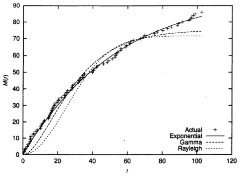
Figure 1: The actual software failure data and the behaviorof estimated

mean

valuefunctions.

$+$CLCJ$\{[1+\lambda(t_{0}+at_{W})]e^{-\lambda(t_{0}+at_{W}\rangle}-[1+\lambda(t_{0}+at_{L})]e^{-\lambda(t_{0}+at_{L})}\}$

.

(30)

For the Rayleigh distribution, it becomes

$\mathrm{C}(70, t_{W})$ $=$ $k_{0}t_{0}+c_{0} \omega[1-\exp\{-\frac{t_{0}^{2}}{2\theta^{2}}\}]+k_{W}t_{W}$

$+c_{W}\omega$

$+c_{L}\omega\{$

$[\exp\{-$$\mathrm{z}$_{$\}-\exp\{-\frac{(t_{0}+at_{W})^{2}}{2\theta^{2}}\}]$}

$\exp\{-\frac{(t_{0}+at_{W})^{2}}{2\theta^{2}}\}-\exp\{-\frac{(t_{0}+at_{L})^{2}}{2\theta^{2}}\}]$ ‘ (31)

Supposethattheunknown parameters inthe software reliability models

are

estimated by the method

of maximumlikelihood,when70 faultdata

are

obtained,namely$t=$

67.374.

Then,we have theestimates

$(\hat{\omega},\hat{\lambda})$

$=$ (98.5188, 1.84e-02) for the exponential model, $(\hat{\omega},\hat{\lambda})$

$=$ (75.1746, 6.46224e-02) for thegamma

model and $(\hat{\omega},\hat{\theta})=$ $(71.6386, 2.45108\mathrm{e}+01)$ for the Rayleigh model. Figure 1 shows the actual software

fault data and the behavior of estimated

mean

value functions. For the other model parameters,

we

assume:

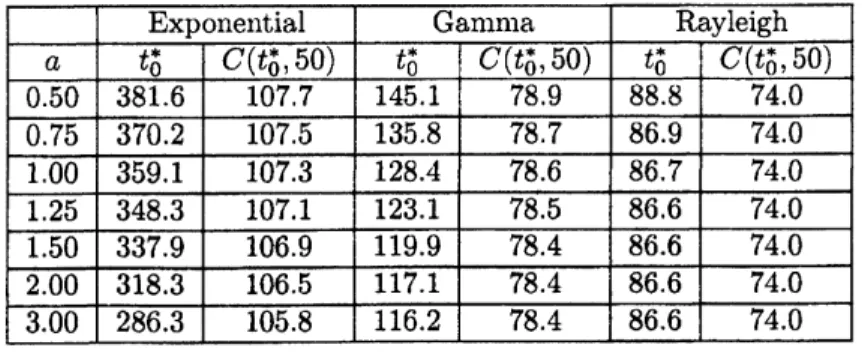
kg $=0.02$, $k_{W}=0.01$,$c_{0}=1.0$, $c_{W}=2.0$, $c_{L}=20.0$ and$t_{L}=$1000.

Ihble 1 presentsthe dependence of the environment factor $a$

on

the optimal testing period$t_{0}^{*}$ when

$t_{W}=50.$ As the environmentfactor_{monotonically increases,} $i.e.$,the operationalcircumstancetends to

be severe, it is observed that the optimal testing period $t$

;

and itsassociated

minimum

total expected

software cost $C(t_{0}^{*}, 50)$ decrease for both exponential and gamma models. For the Rayleigh model, it

is observed thatthe optimal testing periodis hardlyinfluenced byvarying environment factor. Thisis

becausethe goodnessof-fit of theRayleigh model is quite low.

Table2shows thedependence oftheenvironmentfactor$a$

on

the optimal planned maintenance limit

$t\mathrm{i}$ in

case

of$t_{0}=70.$ It is found that the optimal planned

maintenance

limit $t_{W}^{*}$ and the

correspond-ing minimum total expected software cost $C(70, t_{W}^{*})$ decrease

as

theenvironment factor monotonically

increases. Thistendency

can

be explained

as

follows: The residual faults in

software are

detected and

removed at the early stage in the operational phaseasthe operationalenvironmentbecomes

more severe.

Then, the possibility that thesoftware failure

occurs

in the latter stageofthe operational phasebecomes

small. Hence, the implication in which the software developer keeps the

maintenance

team becomes

smaller toward the end of the life cycle.

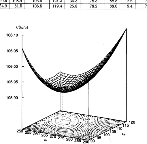
Table 3 examines the dependence of the environment factor $a$

on

the joint optimal policy $(t_{0}^{*},t_{W}^{*})$

combined by testing period and planned maintenance limit. Figure 2 illustrates the behavior of the

78

Table 1: Optimaltesting period for varyingenvironment factor. Exponelltial Gamma $\mathrm{R}^{1}$,ayleigh

$a$ $t_{0}^{*}$ $C(t_{0}^{*}, 50)$ $t_{0}^{*}$ $-C\overline{(}^{-}t_{0}^{*}$,$5\overline{0})^{-}$ $t_{0}^{*}$ $\overline{C(t}_{0}^{*}-$,50)

0.50 381.6

107.7

145.1 78.9 88.8 74.0

0.75

370.2

107.5

135.8 $78.7^{-}$ 86.9 74.0

1.00

359.1

107.3

128.4

_78.6-

86.7

74.0

1.25 348.3

107.

1 123.1

78.5

86.6

74.0

1.50

337.9

106.9

119.9 78.4 86.6

74.0

2.00 318.3

106.5

117.1 86.6 74.0

3.00

286.3

105.8

116.2

78.4

86.6 74.0

Table 2: Optimal planned maintenance limit for varying environment factor. $\overline{\mathrm{E}}\mathrm{x}\mathrm{p}\mathrm{o}\mathrm{n}\mathrm{e}\mathrm{n}\mathrm{t}\mathrm{i}\mathrm{a}\mathrm{l}$ Gamma $\mathrm{R}_{-}*\cdot$$\mathrm{a}^{1}\mathrm{y}1\mathrm{e}\mathrm{i}\mathrm{g}\mathrm{h}$

$a$ $t_{W}^{*}$ $C(70, t_{W}^{*})$ $t_{W}^{*}$ $C(70, t_{W}^{*})$ $t_{W}^{*}$ $C(70, t_{W}^{*})$

0.50

_664.0-

134.8

193.0

83.3 111.9 82.8 0.75

472.1

132.5

137.9

$8_{-}2.7$

77.8

82.4

1.00

369.7

131.3

108.3

82.4

60.0

82.2

1.25

305.5

130.6

89.6 $82.\overline{1}^{-}$ $\overline{4}9.0$ 1.50 261.2 130.1

76.8

82.0

41.5

82.0

2.00 203.7 129.4 60.0 81.8 32.0 81.9 3.00 143.4

128.7

42.3 81.6 22.0 81.8

testing period $t_{0}^{*}$ decreases as the environment factor monotonically increases, but, the monotonicity of the optimal planned maintenance limit $t_{W}^{*}$ is not observed. It is also

seen

that the minimum total

expectedsoftware cost $C(t_{0}^{*}, t_{W}^{*})$ decreases

as

the

environment

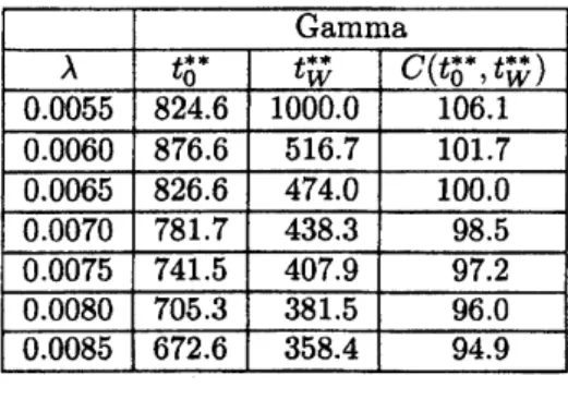
factor monotonically increases.

Tables4, 5 and 6 present the dependence of thesoftware reliability model parameter A

or

$\theta$ on the

joint optimalpolicy$(t_{0}^{*}, t_{W}^{*})$

.

Except forA$=$

0.0055

in thegammamodel, it isobserved thattheoptimal

testing time, optimal planned maintenance limit and its associated minimumtotalexpectedsoftware cost

decrease

as

the fault detection becomes easier.

6

Concluding

Remarks

In this paper,

we

have assumedthat the software developer

was

responsible tothe maintenance service

for all thesoftware failuresthat

occur

duringthe software life cycle underthe maintenancecontract. In order to carry out the maintenance service in the operational phase, the software developer hasto keep

a

software maintenance team. At the

same

time, the management cost inthe operational phase has to be reduced

as

muchas possible, but human

resources

should be utilized effectively. We have called the time length to completethe operational maintenance after the release the planned maintenance limit, and have controlled it in termsofcost-benefit analysis. We have developed the modelwhich considers

the difference in the software execution environment during testing and operational phases using the

same

method

as

the reliability assessment modeling in the operational phase proposed by

Okamura

et

$cd$

.

[12]. Based

on

NHPP

we

haveformulated the totalexpected software cost incurred to the software

developer until the end of

software

life cycle. The optimal testing period (release time) and optimal

planned maintenance limit which minimize the total expected

software cost

have been derived. Then,

throughout the numerical examples,

we

have discussed the joint optimal policy combined by testing

$7\theta$

Table 3: Joint optimal policyfor varying environment factor.

Exponential Gamma Rayleigh

a $0**$ $t_{1}^{**}$ $C(\mathrm{o}t_{W}^{**}**,)$ $0**$ ; $C(t_{0}^{**}t_{W}^{**})-,-$ $t_{0}^{**}$ $t_{W}^{**}$ $C(t_{0}^{*},t^{**})$ $0.50$ 405.0 0.0 107.7 167.4 0.0 78.9 106.3 0.0 73.9

0.75

304.6 159.2 107.3 13 .6 50.4

78.7

94.5 18.4

73.8

1.00 282.6 157.1

-106.8

128.5 49.8 78.6

91.7

18.3 73.8 1.25 272.7 143.3 106.5 125.2 45. 78. 90.4 16.7 73.7 1.50 267.0 129.8 106.2 123.4 41.2 78.4 89. 15.1 73.7 2.00 260.6 108.4 105.9 121.3 34.3 78.3 88.8 12.6 73.7 3.00 254.9 81.5 105. 119.4 25.8 78.2 88.0 9.4 73.6

Figure 2: Behavior of the total expected software costwhen$a=$ 2.00.

Table 4: Jointoptimal policyfor varyingexponentialsoftwarereliability model parameterA.

$\mathrm{E}\mathrm{x}\mathrm{p}\mathrm{o}\mathrm{n}\mathrm{e}\mathrm{n}\underline{\mathrm{t}}\mathrm{i}\mathrm{a}\mathrm{l}$ $\lambda$ $t_{0}^{**}$ $t_{W}^{**}$ $C(t_{0}^{**}, t^{**})$

0.005

735.1

533.6

-122.6

0.010

440.8

263.7

112.0-0.015 320.9 175.8 108.0 0.020 255.1 131.8 106.0 $0^{-}.025$ 213.0 $\overline{1}05.5$ 104.6 0.030 183.6 87.9

103.7

0.035 $16\overline{1}.7$ 75.3 103.1

80

Table 5: Joint optimal policy for varyinggamma software reliability model parameter A.

Gamma

$\lambda$ $t_{0}^{**}$ $t_{W}^{**}$ $C(t_{0}^{**}, t_{W}^{**})$

0.0055

824.6

1000.0

106.1

0.0060 876.6

516.7

101.7

0.0065

826.6

474.0

100.0 $0^{-}.0070$

781.7

438.3 98.5

0.0075

741.5

407.9

97.2 0.0080

705.3

381.5

96.0-0.0085

672.6 358.4 94.9

Table

6:

Joint optimal policy for varying Rayleigh software reliability model parameter $\theta$

.

$\mathrm{R}\mathrm{a}\mathrm{y}\overline{\mathrm{l}}\mathrm{e}\mathrm{i}\mathrm{g}\mathrm{h}$ $\theta$ $t_{0}^{**}$ $t_{W}^{**}$ $C(t_{0}^{**}, t^{**})$ 22.5 83.5 15.2

73.6

23.0

85.2

15.6

73.6

23.5

87.0 16.0

73.7

24.0

88.7

16.3

73.7

24.5 90.4

16.7

73.7

25.0 92.1 17.1

-73.8

25.5

93.7

17.4

73.8

References

[1] K.

Okumoto

and

L. Goel, “Optimum release

time

for software

systems

based

on

reliability

and cost

criteria,” J. Sys. Software, vol. 1, pp. 315 -318, 1980.

[2] $\mathrm{A}.\mathrm{L}$

.

Goel and K. Okumoto, “Time-dependent error-detection rate model

for

software reliability and other performance measures,” IEEETrans. Reliab., vol. R-28,

no.

3, pp. 206-211, 1979.

[3] $\mathrm{H}.\mathrm{S}$

.

Koch and P. Kubat, “Optimalreleasetimeofcomputer software,” IEEE Trans. Software Eng., vol. SE 9,

no.

3, pp. $32\succ 327$,

1983.

[4] Z. Jelinski, and $\mathrm{P}.\mathrm{B}$

.

Moranda, “Software reliability research,” Statistical Computer Performance Evaluation, (W. Freiberger ed.), pp. 465484, Academic Press,New York,

1972.

[5] $\mathrm{D}.\mathrm{S}$

.

Bai and$\mathrm{W}.\mathrm{Y}$

.

Yun, “Optimum number oferrorscorrected before releasingasoftware system,”

IEEE Trans. Reliab., vol. R-37 no. 1, pp. 41-44, 1988.

[6] $\mathrm{W}.\mathrm{Y}$

.

Yun and $\mathrm{D}.\mathrm{S}$

.

Bai, “Optimum software release policy with random life cycle,” IEEE Trans.

Reliab., vol. R-39,

no.

2, pp. 167-170,

1990.

[7] T. Dohi, N. Kaio andS. Osaki, “Optimal software releasepolicieswith debuggingtimelag,”Int. J.

Reliab., QualityandSafety Eng., vol. 4,

no.

3, pp. 241-255,

1997.

[8] M. Kimura, T. Toyota, and

S.

Yamada, “Economic analysis of software release problems with

warranty cost and reliability requirement,” Reliab, _Eng.

_&

_{Sys. Safe., vol. 66,}

_no.

_{1, pp. 49-55,}

1999.

[9] H. Pham and X. Zhang, “A softwarecost modelwith warranty and riskcosts,” IEEETrans.

Com-put., vol. 48,

no.

1, pp. 71-75, 1999.

[10] T. Dohi, H. Okamura, N. Kaio and

S.

Osaki, “The age-dependent optimal warranty policyand

its

application tosoftware maintenance contract,” Proc. 5th$\mathrm{I}\mathrm{n}\mathrm{t}’ 1$ Conf.

on

Probab. Safe. Assess, and

Mgmt. (S. Kondo and K. Furuta,$\mathrm{e}\mathrm{d}\mathrm{s}.$),vol. 4, pp. 2547-2552, University Academy