Asymptotic expansion of the transition probability for non-symmetric random walks on crystal lattices (Spectral and Scattering Theory and Related Topics)
14
0
0
全文
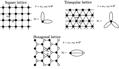
(2) 16. Using the expansion of \cos(n $\theta$) (known asymptotics can be obtained: Theorem 1.1. (Local. as. the. Laplace method),. central limit theorem. the. following long. time. (LCLT)). \displaystyle \lim_{n\rightar ow\infty}\sqrt{2n $\pi$}|p(n, x, y)-e^{-\frac{|x-y|^{2} {2n} |=0. Theorem 1.2. (Asymptotic expansion). p(n, x, y)\displaystyle \sim\frac{1}{\sqrt{2n $\pi$} e^{-\frac{|x-y|^{2} {2n}}(1+c_{1}(x,y)n^{-1}+c_{2}(x, y)n^{-2}\cdots c_{k}(x, y)n^{-k}) Here these limits. and. [14]. As. are. taken. uniformly. for x, y in. some. .. domains. See for instance,. [9], [10]. for the detail.. Spitzer. has mentioned in. [10]. the. ,. periodicity. of \mathbb{Z}^{d}. plays. a. crucial role to obtain. the. asymptotics. This motivated Shirai and Sunada to study the long time asymptotics of a symmetric random walk on a crystal lattice, an abelian covering of a finite graph.. They emphasized. in their articles. ([3], [4], [5], [6], [7], [11], [12], [13]). time behavior of the random walk must not. depend. on. that the. long. the choice of the realization. In. this. geometric point of view, they found that a canonical realization with a flat metric in the asymptotics called a standard realization. Moreover, Sunada presented in [12] the local central limit theorem for the non‐symmetric random walks on crystal lattices. In the proof, the notion of the modified standard realization of the graph into the corresponding continuous space plays a crucial role. In this exposition, we give an outline of the proof of the asymptotic expansion of the transition probability of the non‐symmetric random walks on crystal lattices which is recently proved in [1]. See also [2] for the explicit calculation on the triangular lattice. is. naturally appeared. Discrete harmonic. 2. analysis. on. crystal lattices. We review the. general facts about the discrete harmonic analysis on crystal lattices. all, we give the definition of the crystal lattice. An oriented, locally finite connected graph X=(V, E) is called a crystal lattice if there exists an abelian group $\Gamma$ acting on X freely and its quotient X_{0}= $\Gamma$\backslash X is a finite graph. In other words, X is the abelian cover of a finite graph X_{0} with the covering transformation group $\Gamma$ (see Figure 1). Without loss,of generality, we always assume that $\Gamma$ is torsion‐free ( $\Gamma$\simeq \mathbb{Z}^{d} for some d) by changing the quotient X_{0}. For an oriented edge e\in E the origin and the terminus of e are denoted by o(e) and t(e) respectively. The inverse edge of e\in E is denoted by \overline{e} Let E_{x}=\{e\in E|o(e)=x\} First of. ,. ,. ..
(3) 17. Triangular. Figure. Crystal. $\Gamma$=( $\sigma \sigma$\rangle\underline{\simeq}\mathrm{z}^{2}. lattices. edges with o(e)=x\in V We consider transition probability p:E\rightarrow[0 1 ] with. be the set of $\Gamma$‐invariant. 1:. lattice. random walk. a. .. The transition operator L is. an. operator acting. Then the nstep transition. probability p(n, x, y). from. sum. is taken. over. all. ‐length paths ( e_{1}. n. ,. e2,. .. .. addition, there. exists. a. .. ,. ). x. to y. .. We mention. .. positive function m:V\rightarrow \mathbb{R} such that. then the random walk is said to be measure. by. ,. e_{n} from. p(e)m(o(e))=p(\overline{e})m(t(e)) (e\in E) reversible. X defined. given by. L^{n}f(x)=\displaystyle \sum_{y\in V}p(n, x,y)f(y) (x\in V). a. a. .. to y is. x. on. p(n, x,y):=\displaystyle \sum_{(e1,e2,\ldots \mathrm{e}_{n})},p(e_{1})p(e_{2})\cdots p(e_{n}) in. given by. .. functions. on. Lf(x):=\displaystyle \sum_{\mathrm{e}\in E_{x} p(e)f(t(e). If,. X. ,. \displaystyle \sum_{e\in B_{x} p(e)=1, p(e)+p(\overline{e})>0 (e\in E). where the. on. ,. symmetric (or reversible), and the function m is called Note that m is uniquely determined up to. for the random walk..
(4) 18. multiple. The most canonical symmetric random walk is the simple random probability given by p(e)=(\deg o(e))^{-1}(e\in E) Now let us consider the discrete spectral analysis on X_{0} By the $\Gamma$‐periodicity of the random walk on X the corresponding random walk on X_{0} can be defined. We always assume that the random walk on X_{0} is irreducible, that is, for every x, y\in V_{0} there exists some n=n(x, y)\in \mathbb{N} such that p(n, x, y)>0 We note that the irreducibility on X_{0} holds on X However, the converse does not in general. By the Perron Frobenius theorem, there exists a unique positive function m : V_{0}\rightarrow \mathbb{R} called the invariant probability measure, satisfying \displaystyle \sum_{x\in V_{0}}m(x)=1 and a. constant. walk with the transition. .. .. ,. ,. .. .. ,. m(x)= tLf (x). where. {}^{t}Lf(x)=\displaystyle \sum_{e\in(E_{0})_{x}}p(\overline{e})f(t(e)). invariant. measure m. is. an. ,. the. eigenfunction. (2.1). ,. transposed operator of L It means that positive eigenvalue 1. .. the. of {}^{t}L for the maximal. We put. \tilde{m}(e)=m(o(e))p(e) (e\in E_{0}) When. \tilde{m}(e)=\tilde{m}(\overline{e}). ,. the random walk is said to be. .. (m-) symmetric.. We consider the 0‐chain group. C_{0}(X_{0},\displaystyle \mathb {R})=\{\sum_{x\in V_{0} a_{x}x|a_{x}\in \mathb {R}\} and the 1‐chain group. C_{1}(X_{0},\displaystyle \mathb {R})=\{\sum_{\mathrm{e}\in E_{0} a_{e}e|a_{e}\in \mathb {R}\}, imposed for e\in E_{0} The boundary operator \partial : C_{1}(X_{0},\mathbb{R})\rightarrow C_{0}(X_{0}, \mathbb{R}) is defined by \partial(e) :=t(e)-o(e) The first homology group \mathrm{H}_{1}(X_{0}, \mathbb{R}) is the kernel \mathrm{K}\mathrm{e}\mathrm{r}(\partial)\subset C_{1}(X_{0}, \mathbb{R}) \mathrm{H}_{1}(X_{0},\mathbb{Z}) is also defined by replacing \mathbb{R} by \mathbb{Z}. where the relation \overline{e}=-e is. .. .. .. We define the 0 ‐cochain group. C^{0}(X_{0},\mathbb{R}):=\{f:V_{0}\rightarrow \mathbb{R}\} with the inner. product. \langle f_{1},. f_{2}\displaystyle \rangle_{0}=\sum_{x\in V_{0} f_{1}(x)f_{2}(x). (f_{1}, f_{2}\in C^{0}(X_{0},\mathbb{R})). ,. and the 1‐cochain group. C^{1}(X_{0},\mathbb{R}):=\{ $\omega$:E_{0}\rightarrow \mathbb{R}| $\omega$(\overline{e})=- $\omega$(e)\} with the inner. product. \displaystyle\{$\omega$_{1},$\omega$_{2})_{1}=\frac{1}{2}\sum_{e\inE_{0} $\omega$_{1}(e)$\omega$_{2}(e)($\omega$_{1},$\omega$_{2}\inC^{1}(X_{0},\mathb {R}). ..
(5) 19. A 1‐cocháin is. occasionally called. a. 1‐form. We define the difference operator. on. X_{0}.. d:C^{0}(X_{0}, \mathbb{R})\rightarrow C^{1}(X_{0}, \mathbb{R}) by. df(e) :=f(t(e))-f(o(e)) (e\in E_{0}). ,. and the first cohomology group \mathrm{H}^{1}(X_{0},\mathbb{R}) :=C^{1}(X_{0},\mathbb{R})/{\rm Im}(d) the dual of the first homology group \mathrm{H}_{1}(X_{0},\mathbb{R}). .. \mathrm{H}^{1}(X_{0},\mathbb{R}). Note that. is. .. We define the. homological. direction. by. $\gamma$_{p}:=\displaystyle \sum_{e\in E_{0} \tilde{m}(e)e\in C_{1}(X_{0}, \mathb {R}) \partial$\gamma$_{p}=0. We observe that p. gives. a. $\gamma$_{p}\in \mathrm{H}_{1}(X_{0},\mathbb{R}) walk, i.e., \tilde{m}(e)=\tilde{m}(\overline{e}).. and hence,. symmetric random. .. .. We note that A 1‐form. $\omega$. $\gamma$_{\mathrm{p} =0. only if modified. if and. is said to be. harmonic if. $\delta$_{p} $\omega$(x)+\{$\gamma$_{\mathrm{p} , $\omega$\rangle=0 (x\in V_{0}). (2.2). ,. ($\delta$_{p} $\omega$)(x) :=-\displaystyle \sum_{e\in(E_{0})_{x} p(e) $\omega$(e) and \{$\gamma$_{p}, $\omega$\} :=C_{1}(X_{0},\mathbb{R})\{$\gamma$_{p}, $\omega$\}_{C^{1}(X_{0},\mathbb{R})} is constant as on V_{0} We denote by \mathcal{H}^{1}(X_{0}) the set of modified harmonic 1‐forms, and equip with the inner product \mathcal{H}^{1}(X_{0}) where a. function. \ll$\omega$_{1}, Then the. .. $\omega$_{2}\displaystyle \g :=\sum_{e\in E_{0} $\omega$_{1}(e)$\omega$_{2}(e)\overline{m}(e)-\langle$\gam a$_{p}, $\omega$_{1}\rangle\{$ gam a$_{\mathrm{p},$\omega$_{2}\ ($\omega$_{1}, $\omega$_{2}\in \mathcal{H}^{1}(Xo). corresponding. norm. \Vert\cdot\Vert. is. Lemma. 5.2]),. for every closed. path. By the discrete Hodge‐Kodaira theorem (cf. [7,. \mathrm{H}^{1}(X_{0},\mathbb{Z}). with. \mathcal{H}^{1}(X_{0}). (2.3). given by. \displaystyle \Vert $\omega$\Vert^{2}:=\langle( $\omega,\ \omega$\}\}=\sum_{ $\epsilon$\in E_{0} | $\omega$(e)|^{2}\overline{m}(e)-\{$\gamma$_{p}, $\omega$)^{2} ( $\omega$\in \mathcal{H}^{1}(X0) and. .. we. may. .. identify \mathrm{H}^{1}(X_{0},\mathbb{R}). and. \displaystyle\{$\omega$\in\mathcal{H}^{1}(X_{0})|\int_{\mathrm{c} $\omega$ :=\displaystyle\sum_{i=1}^{n}$\omega$(e_{i})\in\mathb {Z}. c=(e_{1}, \ldots , e_{n}). in. X_{0}\},. on \mathrm{H}^{1}(X_{0},\mathbb{R}) respectively. Using this identification, we obtain an inner product We denote by $\pi$:X\rightarrow X_{0} the covering map, and by $\rho$:\mathrm{H}_{1}(X_{0}, \mathbb{Z})\rightar ow $\Gamma$ the surjective homomorphism associated with the covering map $\pi$ We extend $\rho$ to the surjective linear Then we may consider the injective linear map t_{$\rho$_{\mathb {R} : map $\rho$_{\mathb {R} : \mathrm{H}_{1}(X_{0}, \mathbb{R})\rightar ow $\Gamma$\otimes \mathbb{R} .. .. .. \mathrm{H}\mathrm{o}\mathrm{m}( $\Gamma$, \mathbb{R})\rightar ow \mathrm{H}^{1}(X_{0},\mathbb{R}) by. t_{$\beta$_{\mathbb{R} : $\omega$\in \mathrm{H}\mathrm{o}\mathrm{m}( $\Gamma$,\mathbb{R})}\mapsto{}^{t}$\rho$_{\mathrm{N} ( $\omega$)(\cdot):= $\omega$($\rho$_{\mathbb{R} (\cdot) \in \mathrm{H}^{1}(X_{0}, \mathbb{R}) where maps. \mathrm{H}\mathrm{o}\mathrm{m}( $\Gamma$, \mathb {R}) {}^{t}$\rho$_{1\mathrm{R} and $\rho$_{\mathrm{R} ,. denotes the linear space of we. identify \mathrm{H}\mathrm{o}\mathrm{m}( $\Gamma$,\mathb {R}). ,. homomorphisms of $\Gamma$ into \mathbb{R} Using the subspace Image ({}^{t}$\rho$_{\mathb {R} ) in \mathrm{H}^{1}(X_{0},\mathbb{R}) and. with the. ..
(6) 20. $\Gamma$\otimes \mathbb{R} with the quotient linear subspace of. \mathrm{H}_{1}(X_{0}, \mathbb{R}). .. We denote. t_{$\rho$_{\mathbb{R} ( $\omega$)}\in \mathrm{H}^{1}(X_{0}, \mathbb{R}). on \mathrm{H}^{1}(X_{0}, \mathbb{R}) to product the subspace \mathrm{H}\mathrm{o}\mathrm{m}(\mathrm{F}, \mathb {R}) and then take up the dual inner product \rangle_{atb} on $\Gamma$\otimes \mathbb{R} The flat metric on $\Gamma$\otimes \mathbb{R} induced from this inner product is called the Albanese metric and is denoted by g_{0} This procedure is summarized in the following diagram:. the. by. same. symbol. $\omega$. for. brevity.. We restrict the inner. ,. .. .. ( $\Gamma$\otimes \mathbb{R}, g_{0}) \leftarrow \mathrm{K} \mathrm{H}_{1}(X_{0},\mathbb{R}) 3 dual. \mathrm{X} dual. \mathrm{H}\mathrm{o}\mathrm{m}( $\Gamma$, \mathbb{R}) \mapsto^{\mathrm{B} $\iota$_{ $\rho$} \mathrm{H}^{1}(X_{0},\mathbb{R})\cong(\mathcal{H}^{1}(X0), \cdot\gg) We write. (X, $\Gamma$). Now \mathrm{A}. \mathrm{A}\mathrm{l}\mathrm{b}^{$\Gam a$}. for. ( $\Gamma$\otimes \mathbb{R}/ $\Gamma$\otimes \mathbb{Z}, g_{0}). ,. and call it the $\Gamma$ ‐Albanese torus associated with. .. we. realize X in $\Gamma$\otimes \mathbb{R}. (piecewise linear). map $\Phi$. :. equipped. with the Albanese metric g_{0} in a standard way. a periodic realization of X if it. X\rightarrow $\Gamma$\otimes \mathbb{R} is said to be. satisfies. $\Phi$( $\sigma$ x)= $\Phi$(x)+ $\sigma$\otimes 1 (x\in X, $\sigma$\in $\Gamma$) We may define a special base point x_{*}\in V and. periodic. realization $\Phi$_{0}. :. .. X\rightarrow $\Gamma$\otimes \mathbb{R} by. $\Phi$_{0}(x_{*})=0. for. a. fixed. \displayst le\mathrm{H}\mathrm{o}\mathrm{ }($\Gam a$,\mathrm{R})\langle$\omega,\ Phi$_{0}(x)\rangle_{$\Gam a$\otimes1\mathrm{R}=\int_{x *}^{x}\tilde{$\omega$}($\omega$\in\mathrm{H}\mathrm{o}\mathrm{ }($\Gam a$,\mathb {R}. where \tilde{$\omega$} is the lift of. for. $\omega$={}^{t}$\rho$_{\mathbb{R} ( $\omega$)\in \mathrm{H}^{1}(X_{0},\mathbb{R}). to X. .. (2.4). Here. \displayst le\int_{x *}^{x}\overline{$\omega$}=l\overline{$\omega$}:=\sum_{i=1}^{n}\tilde{$\omega$}(e_{i}). apath c=(e_{1}, \ldots, e_{n}) with o (e_{1})=x_{*} and t(e_{n})=x It should be noted that this integral does not depend on the choice of a path c. One of the special properties of $\Phi$_{0} is that it is a vector‐valued modified‐harmonic .. line. function. on. X in the. sense. that. L$\Phi$_{0}(x)-$\Phi$_{0}(x)=$\rho$_{\mathrm{R}}($\gamma$_{p}) (x\in V) Indeed, for. every. of the transitioh. $\omega$=$\iota$_{$\rho$_{\mathbb{R} ( $\omega$)}\in \mathrm{H}^{1}(X_{0}, \mathbb{R}). probability. p and the. \mathrm{H}\mathrm{o}\mathrm{m}($\Gam a$,\mathrm{R})\langle$\omega$, L$\Phi$_{0}(x)-$\Phi$_{0}(x)\rangle_{ $\Gamma$\otimes \mathbb{R}. the modified. .. harmonicity (2.2), identity (2.4) imply ,. (2.5) $\Gamma$ ‐invariance. \displayst le\sum_{\mathrm{e}\inE_{x}p(e)_{\mathrm{H}\mathrm{a}\mathrm{ }($\Gam a$,\mathb {R})\langle$\omega$, $\Phi$_{0}(t(e) -$\Phi$_{0}(o(e) \rangle_{ $\Gamma$\otimes \mathbb{R} =\displaystyle \sum_{e\in E_{x} p(e)\overline{ $\omega$}(e) =. =\displaystyle\sum_{\mathrm{e}\in(E_{0})_{$\pi$(x)} p(e)$\omega$(e). = -($\delta$_{p} $\omega$)( $\pi$(x)). = \{$\gamma$_{p}, $\omega$\}=\mathrm{H}\circ \mathrm{m}( $\Gamma$,\mathrm{R})\langle $\omega,\rho$_{\mathrm{R} ($\gamma$_{\mathrm{p} )\rangle_{ $\Gamma$\otimes \mathrm{R} (x\in V). ..
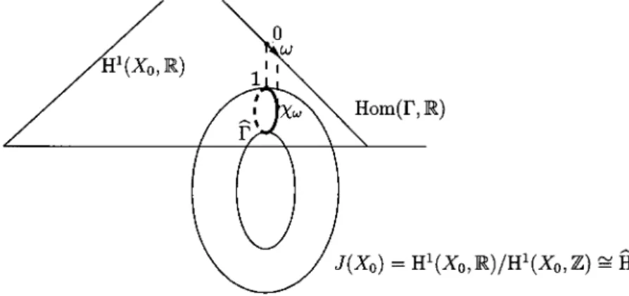
(7) 21. A periodic realization $\Phi$ : X\rightarrow $\Gamma$\otimes \mathbb{R} satisfying (2.5) is said to be modified harmonic. Note that a modified harmonic realization is uniquely determined up to translation. If we equip $\Gamma$\otimes \mathbb{R} with the Albanese metric g_{0} then we call the map $\Phi$_{0} : X\rightarrow( $\Gamma$\otimes \mathbb{R}, g_{0}) the modified standard realization of X We readily check that the piecewise linear interpolation of $\Phi$_{0} by hne segments descends to a piecewise geodesic map $\Phi$_{0} : X_{0}\rightar ow \mathrm{A}\mathrm{l}\mathrm{b}^{ $\Gamma$}. We call $\Phi$_{0} the Albanese map associated with (X, $\Gamma$) Namely, standard realization is a ,. .. .. lift of the Albanese map. In [12], Sunada presented the local central limit theorem random walk. on. lattices stated. crystal. (LCLT). for. non‐symmetric. follows: Let. as. K :=\mathrm{g}.\mathrm{c}.\mathrm{d}.\{\mathrm{n}\in \mathbb{N};\mathrm{p}(\mathrm{n},\mathrm{x},\mathrm{x})\neq 0\} be the. period of the. random walk and. ([12]). Theorem 2.1. Let. V=\square _{k=0}^{K-1}A_{k}. the K ‐partition of V.. x\in A_{i}, y\in A_{j} If n=Kl+j-i, .. p(n,x y)m(y)^{-1}\displayst le\sim\frac{K\mathrm{v}\mathrm{o}1(\mathrm{A}1\mathrm{b}^{$\Gam a$}){(2$\pi$n)^{d/2}e(-\frac{|$\Phi$(x)-$\Phi$(y)-n$\rho$_{\mathrm{R}($\gam a$_{\mathrm{p}\rangle|_{9}^{2}{2n}) Otherwise. p(n, x,y)=0. ,. where. \mathrm{v}\mathrm{o}\mathrm{l}(\mathrm{A}\mathrm{l}\mathrm{b}^{$\Gam a$}). is the volume. of Albr. .. with the Albanse metric. g_{0}.. Asymptotic expansion. 3. Recall that. X=(V, E). probability. covering transformation group $\Gamma$ is a period of the random walk on X We note that we can retake the covering transformation group so that the period of the corresponding random walk on X_{0} has the same period K. is. a. crystal lattice. of the transition in which. torsion free abelian group of rank d and torsion free. Let K be the .. Twisted transition operators. 3.1. We first review Let. \hat{\mathrm{H} _{1}(X_{0}, \mathb {Z}). some. basic results. be the group of with the Jacobian torus. on. the twisted transition operators studied in. unitary characters of \mathrm{H}_{1}(X_{0}, \mathbb{Z}). .. J(X_{0}):=\mathrm{H}^{1}(X_{0},\mathbb{R})/\mathrm{H}^{1}(X_{0}, \mathbb{Z}) by. the. mapping. \mathrm{H}^{1}(X_{0},\mathbb{R})\ni $\omega$\mapsto$\chi$_{ $\omega$}\in\hat{\mathrm{H} _{1}(X_{0}, \mathbb{Z}). ,. where. $\chi$_{ $\omega$}( $\sigma$):=\displaystyle \exp(2 $\pi$\sqrt{-1}\int_{c_{ $\sigma$} $\omega$) ( $\sigma$\in $\Gamma$). We. identify. [3, 4, 8].. \hat{\mathrm{H} _{1}(X_{0}, \mathb {Z}).
(8) 22. and c_{ $\sigma$} is induced Let. a. by. \hat{$\Gam a$}. the above. closed. path. the metric. be the group of. mapping,. X_{0} satisfying $\rho$([\mathrm{c}_{ $\sigma$}])= $\sigma$. in. (2.3). on. \mathrm{H}^{1}(X_{0}, \mathbb{R})(\cong \mathcal{H}^{1} (Xo) ). We. .. equip. a. flat metric. unitary characters of the covering transformation. we can. identify \hat{$\Gam a$}. also. J(X_{0}). on. .. group $\Gamma$. By. .. with the $\Gamma$ ‐Jacobian torus. \mathrm{J}\mathrm{a}\mathrm{c}^{ $\Gamma$}:=\mathrm{H}\mathrm{o}\mathrm{m}( $\Gamma$,\mathb {R})/\mathrm{H}\mathrm{o}\mathrm{m}( $\Gamma$, \mathb {Z}). .. surjective homomorphism $\rho$ : \mathrm{H}_{1}(X_{0}, \mathbb{Z})\rightar ow $\Gamma$ gives rise to an injective homomorphism \mathrm{J}\mathrm{a}\mathrm{c}^{$\Gam a$} into J(X_{0}) We regard \mathrm{J}\mathrm{a}\mathrm{c}^{$\Gam a$} as the flat torus with the metric induced by that on J(X_{0}) The tangent space T_{1}\hat{ $\Gamma$} at the trivial character 1 coincides with \{ $\omega$\in \mathrm{H}^{1}(X_{0},\mathbb{R})|$\chi$_{ $\omega$}\in $\Gamma$ and it is identified with \mathrm{H}\mathrm{o}\mathrm{m}( $\Gamma$,\mathb {R}) (see Figure 2). Since the lattice The canonical. .. .. Figure. \hat{ $\Gamma$}\subset J(X_{0}). 2:. and. group $\Gamma$\otimes \mathbb{Z} in $\Gamma$\otimes \mathbb{R} and the lattice group observe that the $\Gamma$ ‐Albanese torus ,. To. analyze. $\chi$\in\hat{ $\Gamma$}. .. in. ‐step transition probability. n. For each. ,. we. are. dual each. other,. is the dual flat torus of. p(n, x, y). for the random walk. on. the. introduce the twisted transition operator L_{ $\chi$} for a unitary we consider the |V_{0}| ‐dimensional inner product space. $\chi$\in\hat{ $\Gamma$}. ,. \el _{ $\chi$}^{2}= { f X\rightarrow \mathbb{C}|f( $\sigma$ x)= $\chi$( $\sigma$)f(x) :. with the inner. \mathrm{H}\mathrm{o}\mathrm{m}( $\Gamma$, \mathb {R}). .. \mathrm{v}\mathrm{o}\mathrm{l}(\hat{$\Gam a$})=\mathrm{v}\mathrm{o}\mathrm{l}(\mathrm{J}\mathrm{a}\mathrm{c}^{$\Gam a$})=\mathrm{v}\mathrm{o}\mathrm{l}(\mathrm{A}\mathrm{l}\mathrm{b}^{$\Gam a$})^{-1}.. the. crystal lattice X=(V, E) character. \mathrm{H}\mathrm{o}\mathrm{m}( $\Gamma$, \mathb {Z}). \mathrm{A}\mathrm{l}\mathrm{b}^{ $\Gamma$}=( $\Gamma$\otimes \mathb {R}/ $\Gamma$\otimes \mathb {Z},g_{0}). we. \mathrm{J}\mathrm{a}\mathrm{c}^{$\Gam a$} and hence. \mathrm{H}\mathrm{o}\mathrm{m}( $\Gamma$, \mathbb{R})\subset \mathrm{H}^{1}(X_{0}, \mathbb{R}). for $\sigma$\in $\Gamma$ }. product. \displaystyle \langle f, g\}_{ $\chi$}=,\sum_{x\in F}f(x)\overline{g(x)}, where \mathcal{F}\subset V is. independent. a. fundamental domain of X for $\Gamma$. of the choice of. a. .. We note that the inner. fundamental domain \mathcal{F}.. product. is.
(9) 23. As the transition operator L and its transpose {}^{t}L preserve. \el_{$\chi$}^{2} (see [8]), we define the {}^{\mathrm{t} L_{$\chi$} \el _{ $\chi$}^{2}\rightar ow l_{ $\chi$}^{2} by the. l_{ $\chi$}^{2}\rightar ow\el _{ $\chi$}^{2}. and its transposed operator twisted transition operator L_{ $\chi$} : restriction of L and {}^{t}L , respectively. For the trivial character $\chi$=1,. identified with. are. rise to the direct. (L, \ell^{2}(X_{0})). and. ({}^{t}L, \ell^{2}(X_{0})) respectively. ,. The. :. (L_{1}, P_{1}^{2}). family. integral decomposition. ({}^{t}L_{1}, P_{1}^{2}). and. \{L_{ $\chi$}\}_{ $\chi$\in\hat{ $\Gamma$}. gives. (L, P^{2}(X) =\displaystyle \int_{\hat{ $\Gam a$} ^{\oplus}(L_{ $\chi$},l_{ $\chi$}^{2})d $\chi$, where sition. d $\chi$ denotes the normalized Haar measure on \hat{$\Gam a$} As in [8, Section 7], this decompo‐ implies an integral expression of the n‐step transition probability .. p(n, x, y)=\displaystyle \int_{\hat{ $\Gamma$} \langle L_{ $\chi$}^{n}f_{y}, f_{x}\rangle_{ $\chi$}d $\chi$ (n\in \mathb {N}, x, y\in V) f_{x}\in l_{ $\chi$}^{2}. where. is the modified delta function defined. (3.1). ,. by. f_{x}(z):=\left{\begin{ar y}{l $\chi$( \sigma$)&\mathrm{i}\ athrm{f}z=$\sigma$x,\ 0&\mathrm{o}\mathrm{}\ athrm{}\mathrm{e}\mathrm{}\ athrm{w}\mathrm{i}\ athrm{s}\mathrm{e}. \end{ar y}\right. It follows from From this case,. we. note. \langle L_{ $\chi$}^{n}f_{y}, f_{x}\rangle_{ $\chi$}=0(x\in A_{i}, y\in A_{j}, n\neq Kl+j-i). general viewpoint, let us see the case of the that X= $\Gamma$=\mathbb{Z}^{d} and |V_{0}|=1 Moreover,. that. p(n, x, y)=0.. square lattice. graph \mathb {Z}^{d}. .. In this. .. \hat{ $\Gamma$}=\{ $\chi$( $\sigma$)=e^{2 $\pi$\sqrt{-1}\langle $\theta,\ \sigma$)}| $\theta$\in[0, 1)^{d}\}\simeq \mathrm{T}^{d}. Then. we. obtain. \el _{ $\chi$}^{2}=\el _{ $\theta$}^{2}=\mathrm{s}\mathrm{p}\mathrm{a}\mathrm{n}\{e^{2 $\pi$\sqrt{-1}\langle $\theta$,\cdot\rangle}\} and. hence, for f\in P^{2}(X). ,. f(x)=\displaystyle\int_{$\theta$\in\mathrm{F}^{\mathrm{d} a($\theta$)e^{2$\pi$\sqrt{-1}($\theta$,x\rangle}d$\theta$, which is. By. nothing. but the Fourier inversion formula.. virtue of the Perron Frobenius theorem for the random walk with. twisted transition operator L_{ $\chi$} has K ‐simple maximum with eigenfunctions satisfying. eigenvalues $\mu$_{0}( $\chi$). L_{ $\chi$}$\phi$_{k, $\chi$}=$\mu$_{k}( $\chi$)$\phi$_{k, $\chi$}, {}^{t}L_{ $\chi$}$\psi$_{k, $\chi$}=\overline{$\mu$_{k}( $\chi$)}$\psi$_{k, $\chi$}, \{$\phi$_{k, $\chi$}, $\phi$_{k, $\chi$}\rangle_{ $\chi$}=($\phi$_{k, $\chi$},$\psi$_{k, $\chi$}\}_{ $\chi$}=1. Then. we. period K the. note that. $\mu$_{0}(1)=1, $\mu$_{k}( $\chi$)=e^{(\frac{2k $\pi$ \mathcal{F}-\overline{1} {K})}$\mu$_{0}( $\chi$). ,. ,. .. ... ,. $\mu$_{K-1}( $\chi$).
(10) 24. and, for x\in A_{i},. $\phi$_{k, $\chi$}(x)=e^{(\frac{2k_{l} $\pi \Gamma$-\overline{1} {K})}$\phi$_{0, $\chi$}(x) , $\psi$_{k, $\chi$}(x)=e^{(\frac{2kl $\pi$\leftrightar ow-}{K})}$\psi$_{0, $\chi$}(x). (3.2). .. We also note that. \Vert L_{ $\chi$}\Vert\leq 1 (|$\mu$_{k}( $\chi$)|\leq 1). ,. \Vert L_{ $\chi$}\Vert=1\Leftrightarrow $\chi$=1 (|$\mu$_{k}( $\chi$)|=1\Leftrightarrow $\chi$=1) and. \ell_{ $\chi$}^{2}=\oplus_{k=0}^{K-1}\{$\phi$_{k, $\chi$}\}+V_{ $\chi$}, \Vert L_{ $\chi$}f_{V}\Vert<(1- $\epsilon$)\Vert f_{V}\Vert. where. for. f_{V}\in V_{ $\chi$} By (3.1), .. we. obtain. (3.3). p(n, x,y)=L^{n}$\delta$_{y}(x). =\displaystyle\int_{\hat{$\Gam a$}(\sum_{k=0}^{K-1}$\mu$_{k}($\chi$)^{n}$\phi$_{k,$\chi$}(x)\overline{$\psi$_{k,$\chi$}(y)}+\{L_{$\chi$}^{n}\{(f_{y})_{\mathcal{V}_{$\chi$}\},f_{x}\_{$\chi$})d$\chi$ Since we. for. L_{ $\chi$}. preserves. \mathcal{V}_{$\chi$}. and. ,. \Vert L_{ $\chi$}|_{\mathcal{V}_{ $\chi$} \Vert<1- $\epsilon$. for. $\epsilon$>0. some. uniformly. in. .. (3.4). $\chi$\in\hat{ $\Gamma$} (see [3]),. have. some. (3.4),. we. |\displaystyle \int_{\hat{ $\Gam a$} \{L_{ $\chi$}^{n}\{(f_{y})_{v_{ $\chi$} \}, f_{x})_{ $\chi$}d $\chi$|\leq C(1- $\epsilon$)^{n}. constant C. positive. independent of. x. and y. .. (3.5). Therefore. substituting (3.2). into. obtain. p(n,x y)\displaystyle\sim\int_{\hat{$\Gam a$} \sum_{k=0}^{K-1}e(\frac{2k(n-lJ)$\pi$-1}{K})_{$\mu$_{0}(x)^{n}$\phi$_{0,$\chi$}(x)\overline{$\psi$_{0,$\chi$}(y)}d$\chi$}. If. n=Kl+j-i. ,. we. conclude. p(n, x, y)\displaystyle \sim K\int_{ $\Gamma$}$\mu$_{0}( $\chi$)^{n}$\phi$_{0, $\chi$}(x)\overline{$\psi$_{0, $\chi$}(y)}d $\chi$ Using. a. unitary. map. P^{2}(X_{0}). with. l_{$\chi$_{$\omega$}^{2}. given by. f\mapsto s_{ $\omega$}(x)f(x)=e^{2 $\pi$\sqrt{-1}( $\omega,\Phi$_{0}(x)\rangle}f(x) we can. rewrite. $\phi$_{0, $\chi$}. and. $\psi$_{0, $\chi$}. ,. as. $\phi$_{0,$\chi$_{ $\omega$}}(x)=s_{ $\omega$}(x)$\phi$_{ $\omega$}(x) , $\psi$_{0,$\chi$_{ $\omega$}}(x)=s_{ $\omega$}(x)$\psi$_{ $\omega$}(x) where on. $\phi$_{ $\omega$} and $\psi$_{ $\omega$}. P^{2}(X_{0}). is the. defined. (3.6). .. eigenfunction. of the. Harper operator H_{ $\omega$}. ,. and its. adjoint H_{ $\omega$}^{*} acting. by. H_{ $\omega$}f(x_{0}):=\displaystyle \sum_{\mathrm{e}\in(E_{0})_{x_{0} }p(e)\exp(2 $\pi$\sqrt{-1} $\omega$(e) f(t(e) (x_{0}\in V_{0}) H_{ $\omega$}^{*}f(x_{0}):=\displaystyle \sum_{\mathrm{e}\in(E_{0})_{x_{\mathrm{O} }p(\overline{e})\exp(2 $\pi$\sqrt{-1} $\omega$(e) f(t e) (x_{0}\in V_{0}). ,. ,.
(11) 25. respectively. Putting. $\mu$_{0}( $\chi$)=e^{- $\lambda$( $\omega$)}. ,. we. obtain. $\mu$_{0}($\chi$_{ $\omega$})^{n}$\phi$_{0,$\chi$_{ $\omega$} (x)\overline{$\psi$_{0,$\chi$_{ $\omega$} (y)}. =e^{-n$\lambda$($\omega$)}$\phi$_{$\omega$}($\pi$(x) \displaystyle\overline{$\psi$_{(\lrcorner}($\pi$(y) }\exp(2$\pi$\sqrt{-1}\int_{y}^{x}\tilde{$\omega$}). = e^{-n $\lambda$( $\omega$)}$\phi$_{ $\omega$}( $\pi$(x) \overline{$\psi$_{ $\omega$}( $\pi$(y) }\exp(-2 $\pi$\sqrt{-1}\{ $\omega,\ \Phi$_{0}(y)-$\Phi$_{0}(x) ) for x\in A_{i},. (3.7). into. y\in A_{j}, n=Kl+j-i (3.6), we have. and. sufficiently. small. (3.7). $\omega$\in \mathrm{H}\mathrm{o}\mathrm{m}( $\Gamma$, \mathbb{R}) Substituting .. p(n, x,y)\displaystyle \ap rox K\int_{ $\Gamma$}$\mu$_{0}( $\chi$)^{n}$\phi$_{0, $\chi$}(x)\overline{$\psi$_{0, $\chi$}(y)}d $\chi$. =K\displaystyle\inte^{-n$\lambda$($\omega$)}$\phi$_{$\omega$}($\pi$(x) \overline{$\psi$_{$\omega$}($\pi$(y) }e(-2$\pi$\sqrt{-1}\langle$\omega,\Phi$_{0}(y)-$\Phi$_{0}(x)\rangle)\frac{d$\omega$}{\mathrm{v}\mathrm{o}\mathrm{l}(\mathrm{J}\mathrm{a}\mathrm{c}^{$\Gam a$}). =\displayst le\frac{K\mathrm{v}\mathrm{o}1(\mathrm{A}1\mathrm{b}^{$\Gam a$}){n^\frac{d}2 }\int_{\mathrm{H}\mathrm{o}\mathrm{ }($\Gam a$,\mathrm{R})\subset\mathcal{H}^{1}(Xe^{-n$\lambda$(\frac{$\omega$}{\sqrt{n}0) (-2$\pi$\sqrt{-1}(\frac{$\omega$}{\sqrt{n},$\Phi$_{0}(y)-$\Phi$_{0}(x) _{d$\omega$} \phi$_{\frac{$\omega$}{\sqrt{n} ($\pi$(x)\overline{$\psi$_{\frac{$\omega$}{\sqrt{n} ($\pi$(y)}e.. In order to obtain the desired of. $\lambda$( $\omega$) $\phi$_{$\omega$} ,. and. long. time. asymptotics of p(n, x, y). ,. we. need derivatives. $\psi$_{ $\omega$}.. Lemma 3.1 For. $\omega$\in \mathrm{H}\mathrm{o}\mathrm{m}( $\Gamma$, \mathbb{R}). ,. Let. $\lambda$(t) := $\lambda$(t $\omega$). .. For any k\in \mathrm{N} ,. if necessary, for any 1\leq i\leq k the i‐th derivatives $\lambda$^{(i)}(0) coefficient homogeneous polynomials of \sqrt{-1} $\omega$ In particular,. tions s_{ $\omega$} ,. ,. changing eigensec‐. are. the i‐th order real. .. $\lambda$(0) $\lambda$'(0). $\lambda$''(0). $\lambda$^{(3)}(0). =. 0,. =. -2 $\pi$\sqrt{-1}\{$\gamma$_{p}, $\omega$\rangle,. =. =. 4$\pi$^{2}(\displaystyle \sum_{e\in E_{0} p(e) $\omega$(e)^{2}m(o(e) -\{$\gamma$_{p}, $\omega$\}^{2})=4$\pi$^{2}\Vert $\omega$\Vert^{2}, 8$\pi$^{3}\displaystyle \sqrt{-1}\sum_{e\in E_{0} p(e) $\omega$(e)^{3}m(o(e) -24$\pi$^{2}\sqrt{-1}\Vert $\omega$\Vert^{2}\{$\gamma$_{p}, $\omega$\rangle-8$\pi$^{3}\sqrt{-1}\langle$\gamma$_{\mathrm{p} , $\omega$\}^{3} -6 $\pi$\displaystyle \sqrt{-1}|V_{0}|^{1/2}\sum_{e\in E_{0} p(e) $\omega$(e)d$\phi$_{0}' (e)m(o(e) -16$\pi$^{4}\displaystyle \sum_{e\in E_{0} p(e) $\omega$(e)^{4}m(o(e) +48$\pi$^{4}\mathrm{H} $\omega$\Vert^{4} +64$\pi$^{4}\displaystyle \langle$\gam a$_{p}, $\omega$\rangle\sum_{\mathrm{e}\in E_{0} p(e) $\omega$(e)^{3}m(o e) .-96$\pi$^{4}\{$\gam a$_{p}, $\omega$\rangle^{2}\Vert $\omega$\Vert^{2}-48$\pi$^{4}($\gam a$_{\mathrm{p} , $\omega$\}^{4} -48$\pi$^{2}|V_{0}|^{1/2}\displaystyle \langle$\gamma$_{p}, $\omega$\}\sum_{\mathrm{e}\in E_{0} p(e) $\omega$(e)d$\phi$_{0}'(e)m(o(e) ,. $\lambda$^{(4)}(0). =. +24$\pi$^{2}|V_{0}|^{1/2}\displaystyle \sum_{e\in E_{\mathrm{o} }p(e) $\omega$(e)^{2}($\phi$_{0}' (t(e) -\sum_{z\in V_{0} $\phi$_{0}' (z)m(z) m(o(e) -8 $\pi$\displaystyle \sqrt{-1}|V_{0}|^{1/2}\sum_{e\in E_{0} p(e) $\omega$(e)d$\phi$_{0}^{(3)}(e)m(o(e). ..
(12) 26. Remark 3.2. Differentiating. both sides. of H_{t}^{*}$\psi$_{\mathrm{t} =\exp(-\overline{$\lambda$_{(v}(t)})$\psi$_{t} four. times in t at. t=0,. also obtain. we. $\lambda$^{(3)}(0). 8$\pi$^{3}\displaystyle \sqrt{-1}\sum_{e\in E_{0} p(e) $\omega$(e)^{3}m(o(e) -24$\pi$^{2}\sqrt{-1}\Vert $\omega$\Vert^{2}\langle$\gamma$_{p}, $\omega$\}-8$\pi$^{3}\sqrt{-1}\langle$\gamma$_{p}, $\omega$\rangle^{3} +12$\pi$^{2}|V_{0}|^{-1/2}\displaystyle \sum_{e\in E_{0} p(e) $\omega$(e)^{2}\overline{$\psi$_{0}'(o(e) },. =. and. $\lambda$^{(4)}(0) = -16$\pi$^{4}\displaystyle \sum_{\mathrm{e}\in E_{0} p(e) $\omega$(e)^{4}m(o(e) +48$\pi$^{4}\Vert $\omega$\Vert^{4} +64$\pi$^{4}\displaystyle \langle$\gamma$_{p}, $\omega$)\sum_{e\in E_{0} p(e) $\omega$(e)^{3}m(o(e) -96$\pi$^{4}\{$\gamma$_{p}, $\omega$\}^{2}\Vert $\omega$\Vert^{2} -48$\pi$^{4}\displaystyle \{$\gamma$_{p}, $\omega$\}^{4}-96$\pi$^{3}\sqrt{-1}|V_{0}|^{-1/2}\{$\gamma$_{p}, $\omega$\}\sum_{e\in E_{0} p(e) $\omega$(e)^{2}\overline{$\psi$_{0}'(o(e) } +32$\pi$^{3}\displaystyle \sqrt{-1}|V_{0}|^{-1/2}\sum_{\mathrm{e}\in E_{0} p(e) $\omega$(e)^{3}\overline{$\psi$_{0}'(o(e) }. +24$\pi$^{2}|V_{0}|^{-1/2}\displaystyle \sum_{\mathrm{e}\in E_{0} p(e) $\omega$(e)^{2}($\psi$_{0}'(o(e) -\sum_{z\in V_{0} $\psi$_{0}'(z)\cdot m(o(e) ). Lemma 3.3 \mathrm{N} ,. For $\omega$\in \mathrm{H}\mathrm{o}\mathrm{m}( $\Gamma$, \mathbb{R}). changing eigensections. and. $\psi$_{0}^{(i)}. are. the i‐th order. ,. let. $\phi$_{t}(x_{0})=$\phi$_{t $\omega$}(x)_{0}. and. $\psi$_{t}(x_{0})=$\psi$_{tv}((x_{0}). .. .. For any k\in. if necessary, for any 1\leq i\leq k the i‐th derivatives$\phi$_{0}^{(i)}(x_{0}) real coefficient homogeneous polynomials of \sqrt{-1} $\omega$ In partic‐. s_{ $\omega$} ,. ,. .. ular,. $\phi$_{0}(x_{0})=|V_{0}|^{-1/2}, Furthermore. and. $\psi$Ó. is. a. $\psi$_{0}(x_{0})=|V_{0}|^{1/2}m(x_{0}). purely imaginary‐valued first. ,. $\phi$Ó(xo) =0. order. are. real‐valued second oder. .. polynomial of $\omega$ satisfying. \left{\begin{ar y}{l (I-tL)$\psi$\'{O}(xo)=2$\pi sqrt{}-l|V01/2(\sum_{\ athrm{e}\in(E_{0}) x_{0}p(\overlin{e})$\omega$(e)mt(e)\ -m(x_{0})\sum_{\ athrm{e}\inE_{0}p(\overlin{e})$\omega$(e)mt(e)\ sum_{z\inV_{0} $\psi$\'{O}(z)=0, \end{ar y}\right.. $\phi$Ó and $\psi$Ó. (x_{0}\in V_{0}). (x_{0}\in V_{0}). polynomials of $\omega$ satisfying ,. \left{\begin{ar y}{l (I-L)$\phi$_{0}'(x_{0})=-4$\pi^{2}|V_{0}|^-1/2}(\sum_{\ athrm{e}\in(E_{0}) x_{0}p(e)$\omega$(e)^{2}\ -\sum_{\ athrm{e}\inE_{0}p(e)$\omega$(e)^{2}m(oe) \ sum_{z\inV_{0} $\phi$\'{O}(z)=0 \end{ar y}\right.. (x_{0}\in V_{0}).
(13) 27. and. \left{bginary}{l (I-^tL)$\psi_{0}'(x )=4$\pisqrt{-1}(\um_ein(E{0})_xp(\overlin{})$\omega()$\psi_{0}'(te)+\$gam _{p}0,$\omega}$\psi'{O}(mathr{x}\mathr{o})\ -4$pi^{2}(\sum_ein(E{0})_x\mathr{O}p(\overlin{})$\omega()^{2}$\psi_0(le)\ -m(x_{0})\sumeinE_{0}p(\overlin{})$\omega()^{2}$\psi_0(te)x_{0}\inV )\ sum_{z\inV0}$\psi'{O}(z)=-|V_0\sum{zinV_0}$\phi'{O}(z)m, \end{ary}\ight.. respectively.. Applying. the Fourier. Theorem 3.4. ([1], [2]). analysis, Let. conclude the. we. following:. x\in A_{ $\iota$} and y\in \mathcal{A}_{j} If n=Kl+j-i, .. (2 $\pi$ n)^{d\oint 2}p(n, x,y)m(y)^{-1}. |$\Phi$_{0}(x)-$\Phi$_{0}(y)-n$\rho$_{\mathrm{R} ($\gam a$_{\mathrm{p} )|_{90)}^{2}(1+a_{1}(x,y;$\gam a$_{p})n^{-1}). \sim K\mathrm{v}\mathrm{o}\mathrm{l}(\mathrm{A}\mathrm{l}\mathrm{b}^{ $\Gamma$})e(If n\neq Kl+j-i. ,. then. p(n, x, y)=0. ,. as n\rightarrow\infty.. where. a_{1}( $\pi$(x), $\pi$(y),$\gamma$_{p};$\Phi$_{0}(y)-$\Phi$_{0}(x)-n$\rho$_{\mathbb{R} ($\gamma$_{p})). =\displaystyle\frac{m($\pi$(y) ^{-1} {2$\pi$}\sum_{l=1}^{d}\mathrm{q}_{i}($\Phi$_{0}(y)-$\Phi$_{0}(x)-n$\rho$_{\mathrm{R} ($\gam a$_{p}) _{i}. +\displaystyle\frac{1}{16$\pi$^{3}\sum_{x,j=1}^{d}\mathrm{q}_{ij}($\Phi$_{0}(y)-$\Phi$_{0}(x)-n$\rho$_{\mathrm{R}($\gam a$_{p}) _{j}-\frac{m($\pi$(y) ^{-1}{8$\pi$^{2}\sum_{i=1}^{d}\mathrm{q}_{i} -\displaystyle\frac{m($\pi$(y)^{-1}{32$\pi$^{4}\sum_{i,j=1}^{d}\mathrm{q}_{i}\mathrm{q}_{ij_{\hat{J} -\frac{1} 28$\pi$^{4}\sum_{l,j=1}^{d}\mathrm{q}_{ij}-\frac{5}1536$\pi$^{6}\sum_{i,jk=1}^{d}\mathrm{q}_{ij}\mathrm{q}_{jk }. with. some. coefficients q_{ $\alpha$}=\mathrm{q}_{ $\alpha$}( $\pi$(x), $\pi$(y);$\gamma$_{\mathrm{p}})( $\alpha$=($\alpha$_{1}, \ldots , $\alpha$_{r})\in\{1, \ldots,d\}^{r},r=1, \ldots, 4). References [1]. S. Ishiwata, H. Kawabi and M. Kotani: Long time asymptotics of non‐symmetric random walks on crystal lattices, preprint. http: // arxiv. \mathrm{o}\mathrm{r}\mathrm{g}/\mathrm{a}\mathrm{b}\mathrm{s}/1510.05102. [2]. S. Ishiwata, H. Kawabi and T. Teruya: An explicit effect on non‐symmetry of random walks on the triangular lattice, Math. J. Okayama Univ. 57 (2015), pp.129‐148.. [3]. M. Kotani: An. asymptotic of the large deviation for random walks. Contemp. Math. 347 (2004),. pp. 141‐152.. on a. crystal lattice,. ..
(14) 28. [4]. M. Kotani and T. Sunada:. for. [5]. the heat. Albanese maps and off diagonal long time Phys. 209 (2000), pp. 633‐670.. M. Kotani and T. Sunada:. Standard realizations. maps, Trans. Amer. Math. Soc. 353. [6]. M. Kotani and T. Sunada:. (2003), [7]. [9]. (2000),. of crystal. lattices via harmonic. pp. 1‐20.. Spectral geometry of crystal lattices, Contemp.. Math. 338. pp. 271‐305.. M. Kotani and T. Sunada:. crystal lattice,. [8]. asymptotics. kernel Comm. Math.. Math. Z. 254. Large. (2006),. deviation and the. tangent. cone. at. infinity of. a. pp. 837‐870.. M.. Kotani, T. Shirai and T. Sunada: Asymptotic behavior of the transition probability of a random walk on an infinite graph, J. Funct. Anal. 159 (1998), pp. 664‐689.. G. Lawler, V. Limic: Ramdom Walk: A Modern Introduction,. Cambridge Studies. in. Advanced Mathematics 123, 2010.. [10]. F.. [11]. T. Sunada:. Spizter: Principles of Random Walk, Princeton, NJ:. Proc.. [12]. D. Van.. Nostrand, 1964.. Discrete geometric analysis, Analysis on graphs and its applications, Sympos. Pure Math. 77, Amer. Math. Soc., Providence, RI, 2008, pp. 51‐83.. T. Sunada:. Discrete geometric. analysis,. Lecture slide at Institut Henri Poincaré. (2002), University (2006), (2007). http: / \mathrm{w}\mathrm{w}\mathrm{w} newton. ac. uk/programmes/AGA/discrete Humboldt. ences. [13]. T. Sunada:. [14]. W. Woess:. Isaac Newton Institute for Mathematical Sci‐. .. text‐. pdf. Topological Crystallography: With a View Towards Discrete Geometric Analysis, Surveys and Tutorials in the Applied Mathematical Sciences 6, Springer Japan, 2013. Random Walks. Mathematics 138.. on Infinite Graphs and Groups, Cambridge Cambridge University Press, Cambridge, 2000.. Tiracts in.
(15)
図
関連したドキュメント
A second way involves considering the number of non-trivial tree components, and using the observation that any non-trivial tree has at least two rigid 3-colourings: this approach
[Tetali 1991], and characterises the weights (and therefore the Dirichlet form) uniquely [Kigami 1995]... RESISTANCE METRIC, e.g. equipped with conductances) graph with vertex set V
5. Scaling random walks on graph trees 6. Fusing and the critical random graph 7.. GROMOV-HAUSDORFF AND RELATED TOPOLOGIES.. compact), then so is the collection of non-empty
We study the local dimension of the invariant measure for K for special values of β and use the projection to obtain results on the local dimension of the Bernoulli
The proof uses a set up of Seiberg Witten theory that replaces generic metrics by the construction of a localised Euler class of an infinite dimensional bundle with a Fredholm
These upper right corners are hence the places that are responsible for the streets of these lower levels, on these smaller fields (which again are and remain blocks).. The next
5. Scaling random walks on graph trees. Fusing and the critical random graph 7. Local times and cover times.. GROMOV-HAUSDORFF AND RELATED TOPOLOGIES.. compact), then so is
We study the classical invariant theory of the B´ ezoutiant R(A, B) of a pair of binary forms A, B.. We also describe a ‘generic reduc- tion formula’ which recovers B from R(A, B)
