Pyramidal traveling
fronts
in
the
Allen-Cahn
equations
Masaharu Taniguchi
*Department
of
Mathematical and Computing SciencesTokyo Institute
of
TechnologyO-okayama 2-12-1-W8-38, Tokyo 152-8552, Japan
October
30,
2008
Abstract
Pyramidal traveling fronts in the Allen-Cahn equations have
been studied in the three-dimensional whole space. For a given
admissible pyramid a pyramidal traveling front is uniquely
deter-mined and it is asymptotically stable under the condition that given
perturbations decay at infinity. A pyramidal traveling front is a
combination of planar fronts on the lateral surfaces. Also it is a
combination of two-dimensional V-form waves associated with the
edges of a pyramid.
AMS Mathematical Classifications: $35K57,35B35$
Key words: pyramidal traveling wave, Allen-Cahn equation, stability
1
Introduction
For one-dimensional traveling
waves
in the Allen-Cahn equation or theNagumo equation so many works have been studied. See [1, 4, 9, 10, 2]
and so on. In the two-dimensional plane or higher dimensional spaces the
simplest traveling waves are planar ones. Recently non-planar traveling
waves
in the whole space have been studied by [17, 18, 7, 8, 12, 3, 21, 22]and so on. For non-planar traveling waves researchers are interested in
the shapes of the contour lines or surfaces. Constructing traveling waves
with new shapes is an attracting motivation of the mathematical research.
The mathematical study on these multi-dimensional traveling
waves
willgive information for chemists
or
biochemists to study multi-dimensionalchemical waves or
nerve
transmission phenomena in future.The stability of planar traveling
waves
have been studied by [14, 13,23, 15] and so on. The existence and stability of two-dimensional V-form
waves are
studied by [17, 18, 7, 8, 12]. The existence and the uniqueness andasymptotic stability of pyramidal traveling waves
are
studied in [21, 22].In this paper
we
consider the following equation$\frac{\partial u}{\partial t}=\triangle u+f(u)$ in $\mathbb{R}^{3},$ $t>0$,
$u|_{t=0}=u_{0}$ in $\mathbb{R}^{3}$.
A given function $u_{0}$ belongs to $BU(\mathbb{R}^{3})$
.
Here $BU(\mathbb{R}^{3})$ is the space ofbounded uniformly continuous functions from $\mathbb{R}^{3}$
to $\mathbb{R}$ with the supremum
norm. The Laplacian $\triangle$ stands for
$\partial^{2}/\partial x^{2}+\partial^{2}/\partial y^{2}+\partial^{2}/\partial z^{2}$. We study
nonlinear terms of
bistable
type including cubicones.
This equation iscalled the Allen-Cahn equation or the Nagumo equation.
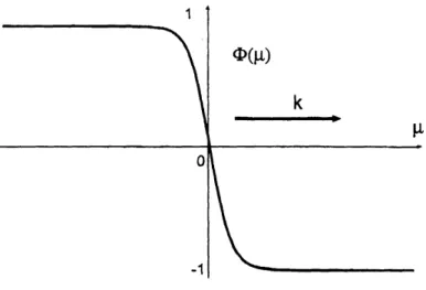
In the one-dimensional space, let $\Phi(x-kt)$ be
a
traveling wave thatconnects two stable equilibrium states $\pm 1$ with speed $k$. By putting
$\mu=$
x–kt, $\Phi$ satisfies
$-\Phi’’(\mu)-k\Phi’(\mu)-f(\Phi(\mu))=0$ $-\infty<\mu<\infty$,
(1)
$\Phi(-\infty)=1$, $\Phi(\infty)=-1$.
To fix the phase
we
set $\Phi(0)=0$.
See Figure 1.The following is the assumptions
on
$f$ in this paper.(Al) $f$ is of class $C^{1}[-1,1]$ with $f(\pm 1)=0$ and $f’(\pm 1)<0$.
(A2) $\int_{-1}^{1}f>0$ holds true.
Figure 1: One-dimensional traveling wave $\Phi$
(A4) There exists $\Phi(\mu)$ that satisfies (1) for some $k\in \mathbb{R}$.
We note that $k>0$ follows from (A2) and (A4).
For
$f(u)=-(u+1)(u+a)(u-1)$
with a given constant $a\in(0,1)$,$\Phi(\mu)=-\tanh(\mu/\sqrt{2})$ satisfies (Al)$-(A4)$ for $k=\sqrt{2}a$. Another simple
example is as follows. Let $G(u)\in C^{2}(\mathbb{R})$ satisfy
$G(\pm 1)=0$, $G’(\pm 1)=0$, $G”(\pm 1)>0$
$G(s)>0$ if $s^{2}\neq 1$,
$\max\{0,\sup_{s<-1}\frac{G’(s)}{\sqrt{2G(s)}}\}<\inf_{s>1}\frac{G’(s)}{\sqrt{2G(s)}}$,
and let $f(u)$ be given by
$f(u)=-G’(u)+k\sqrt{2G(u)}$
for any constant $k$ with
$\max\{0,\sup_{s<-1}\frac{G’(s)}{\sqrt{2G(s)}}\}<k<\inf_{s>1}\frac{G’(s)}{\sqrt{2G(s)}}$,
Then $\Phi(\mu)$ given by
satisfies $(A1)-(A4)$.
For more examples of one-dimensional traveling
waves see
[4, 1, 2, 3, 21].We adopt the moving coordinate of speed $c$ toward the z-axis without
loss of generality. We put $s=z– ct$ and $u(x, y, z, t)=w(x, y, s, t)$. We
denote $w(x, y, s, t)$ by $w(x, y, z, t)$ for simplicity. Then we obtain $w_{t}-w_{xx}-w_{yy}-w_{zz}-cw_{z}-f(w)=0$ $in\mathbb{R}^{3}in\mathbb{R}^{3},$ $t>0$,
(2)
$w|_{t=0}=u_{0}$
Here$w_{t}$ stands for $\partial w/\partial t$ and
so
on. We write the solutionas
$w(x, y, z, t;u_{0})$.
If $v$ is
a
travelingwave
with speed $c$, itsatisfies
$\mathcal{L}[v]def=-v_{xx}-v_{yy}-v_{zz}-\sigma u_{z}-f(v)=0$ in $\mathbb{R}^{3}$
.
(3)We assume
$c>k$
throughout this paper. Since the curvature often accelerates the speed,
one has many travelingwaves if $c>k$. As far as the author knows, it is an
open problem to prove the existence or non-existence of traveling waves if
$c<k$
.
Let $n\geq 3$ be a given integer. We put
$\tau^{d}=^{ef}\frac{\sqrt{c^{2}-k^{2}}}{k}>0$. (4)
Assume $(A_{j}, B_{j})\in \mathbb{R}^{2}$ satisfies
$A_{j}^{2}+B_{j}^{2}=1$ for all $j=1,$
$\ldots,$ $n$ (5) and $A_{j}B_{j+1}-A_{j+1}B_{j}>0A_{n}B_{1}-A_{1}B_{n}>0$
.
(6) $1\leq j\leq n-1$, Now$\nu_{j}^{d}=^{ef}\frac{1}{\sqrt{1+\tau^{2}}}(\begin{array}{l}-\tau A_{j}-\tau B_{j}1\end{array})$
is the unit normal vector of a surface $\{z=\tau(A_{j}x+B_{j}y)\}$
.
We put$h_{j}(x, y)$ $def=$ $\tau(A_{j}x+B_{j}y)$ ,
$h(x, y)$ $def=$
Then $z=h(x, y)$ gives
a
reverse
pyramid in $\mathbb{R}^{3}$. We call it simply a pyramidhereafter. We set
$\Omega_{j}=\{(x, y)|h(x, y)=h_{j}(x, y)\}$ ,
and obtain
$\mathbb{R}^{2}=\bigcup_{j=1}^{n}\Omega_{j}$
.
We locate $\Omega_{1},$ $\Omega_{2},$
$\ldots,$
$\Omega_{n}$ counterclockwise. To
ensure
this locationwe
as-sumed (6). Now the lateral surfaces of a pyramid are given by
$S_{j}=\{(x, y, h_{j}(x, y))\in \mathbb{R}^{3} I (x, y)\in\Omega_{j}\}$
for $j=1,$ $\ldots,$ $n$. We put
$\Gamma_{j}^{d}=^{ef}\{\begin{array}{l}S_{j}\cap S_{j+1} if 1\leq j\leq n-1,S_{n}\cap S_{1} if j=n.\end{array}$
Then $\Gamma_{j}$ represents an edge of a pyramid. Also $\Gamma^{d}=^{ef}\bigcup_{j=1}^{n}\Gamma_{j}$
represents the set of all edges. See Figure 2.
By using $(A_{j}, B_{j})$ with $A_{j}^{2}+B_{j}^{2}=1$, Equation (3) has a solution
$\Phi((k/c)(z-h_{j}(x, y)))$ . It is called
a
planar traveling front associated withthe lateral surface $S_{j}$. Now we put
$\underline{v}(x, y, z)^{d}=^{ef}\Phi(\frac{k}{c}(z-h(x, y)))=\max_{1\leq j\leq n}\Phi(\frac{k}{c}(z-h_{j}(x, y)))$ .
We define
$D(\gamma)^{d}=^{ef}\{(x,$
$y,$ $z)\in \mathbb{R}^{3}|$ dist$((x,$$y,$ $z),$ $\Gamma)\geq\gamma\}$ (8)
for $\gamma\geq 0$.
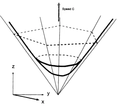
The existence of pyramidal traveling fronts is proved in [21]. See
Fig-ure
3.Theorem 1 ([21]) Let $c>k$ and let $h(x, y)$ be given by (7). Under the
assumptions $(Al),$ (A 2), (A 3) and $(A4)$ there exists a solution $V(x, y, z)$
to (3) with
Figure 2: The edge lines $\Gamma$
Moreover one has
$V_{z}(x, y, z)<0$, $\Phi(\frac{k}{c}(z-h(x, y)))<V(x, y, z)<1$
for
all $(x, y)z)\in \mathbb{R}^{3}$.
The following theorem is the main assertion on the uniqueness and the
stability of pyramidal traveling fronts.
Theorem 2 ([22]) In addition to the assumptions as in Theorem 1 $\sup-$
pose
$\lim_{\gammaarrow+\infty}\sup_{(x,y,z)\in D(\gamma)}|u_{0}(x, y, z)-V(x, y, z)|=0$
.
(10)Then
$\lim_{tarrow+\infty}\sup_{(x,y\}z)\in \mathbb{R}^{3}}|u(x,$ $y$, $z$
– $ct$, $t)-V(x, y, z)|=0$
holds true. Especially $V(x, y, z)$ as in Theorem 1 is uniquely determined
Figure 3: The pyramidal traveling wave $V$
If $u_{0}$ satisfies
$\lim_{Rarrow+\infty}\sup_{x^{2}+y^{2}+z^{2}\geq R^{2}}|u_{0}(x, y, z)-V(x, y, z)|=0$,
it also satisfies (10). Thus the theorem also asserts that a pyramidal
travel-ing wave $V$ is asymptotically stable globally in space if a given fluctuation
decays at infinity. The asymptotic stability is valid for a weaker condition
(10). This
means
that $V$ is robust for fluctuations added on edges. Now$V$ as in Theorem 1 can be called the pyramidal traveling wave associated
with a pyramid $z=h(x, y)$, since it is uniquely determined.
2
Acknowledgements
The author expresses his gratitude to the organizers of a RIMS Meeting
“Viscosity Solutions ofDifferential Equations and Related Topics” He also
expresses his sincere gratitude to Prof. Hirokazu Ninomiya of Ryukoku
University, Dr. Mitsunori Nara, Prof. Hiroshi Matano in University of
Tokyo, Prof. Wei-Ming Ni in University of Minnesota for many discussions
and encouragements. This work was supported by Grant-in-Aid for
3
Preliminaries
Under the assumption (Al) and (A4), $\Phi(\mu)$
as
in (1) satisfies$\Phi’(\mu)<0^{1}$ for all $\mu\in \mathbb{R}$, (11)
$\max\{|\Phi’(\mu)|, |\Phi’’(\mu)|\}\leq K_{0}\exp(-\kappa_{0}|\mu|)$ . (12) Here $K_{0}$ and $\kappa_{0}$
are
some
positive constants. See Fife andMcLeod [4] for
the proof.
IFhrom the assumptions on $f$ there exists apositive constant $\delta_{*}(0<\delta_{*}<$
$1/4)$ with
$-f’(s)>\beta$ if $|s+1|<2\delta_{*}$ or $|s-1|<2\delta_{*}$,
where
$\beta^{d}=^{ef}\frac{1}{2}\min\{-f’(-1), -f’(1)\}>0$
.
Then for all $\delta\in(0, \delta_{*})$ we have
$-f’(s)>\beta$ if $|s+1|<2\delta$ or $|s-1|<2\delta$
.
We state the uniqueness and stability ofatwo-dimensional V-form front
in the
two-dimensional
plane. See Figure 4. Let $\tilde{w}(\xi, \eta, t;\tilde{w}_{0})$ be thesolu-tion of
$\tilde{w}_{t}-\tilde{w}_{\zeta\xi}-\tilde{w}_{\eta\eta}-s\tilde{w}_{\eta}-f(\tilde{w})=0$ for $(\xi, \eta)\in \mathbb{R}^{2},$ $t>0$,
$w(\xi, \eta, 0)=\tilde{w}_{0}(\xi, \eta)$ for $(\xi, \eta)\in \mathbb{R}^{2}$
for a given bounded $\tilde{w}_{0}\in C^{1}(\mathbb{R}^{2})$
.
Theorem
3 (Two-dimensional traveling V-form fronts [17],[18]) Forany $s\in(k, +\infty)$, there exists unique $v_{*}(\xi, \eta;s)$ that
satisfies
$-(v_{*})_{\xi\xi}-(v_{*})_{\eta\eta}-s(v_{*})_{\eta}-f(v_{*})=0$
for
$(\xi, \eta)\in \mathbb{R}^{2}$,$\lim_{Rarrow\infty_{\xi^{2}}}\sup_{+\eta^{2}>R^{2}}|v_{*}(\xi, \eta)-\Phi(\frac{k}{s}(\eta-\frac{\sqrt{s^{2}-k^{2}}}{k}|\xi|))|=0$
.
(13)One has
$\Phi(\frac{k}{s}(\eta-\frac{\sqrt{s^{2}-k^{2}}}{k}|\xi|))<v_{*}(\xi, \eta)$
for
$(\xi, \eta)\in \mathbb{R}^{2}$, (14)Figure 4: Contour lines of a two-dimensional V-form wave $v_{*}(x,y)$ ([17]).
The following convergence
$\lim_{tarrow+\infty}\Vert w(\xi, \eta, t)-v_{*}(\xi, \eta)\Vert_{L^{\infty}(\mathbb{R}^{2})}=0$
holds true
for
any boundedfunction
$\tilde{w}_{0}\in C^{1}(\mathbb{R}^{2})$ with$\lim_{Rarrow\infty_{\xi^{2}}}\sup_{+\eta^{2}>R^{2}}|\tilde{w}_{0}(\xi, \eta)-v_{*}(\xi, \eta)|=0$
.
See also Hamel, Monneau and RoquejofFre [7, 8]. This $v_{*}$ can be
called the two-dimensional traveling V-form front associated with (13)
since it is uniquely determined. We call the $\eta$-axis the traveling
direc-tion of $v_{*}(\xi, \eta;s)$. This theorem asserts the asymptotic stability of $v_{*}$ for
any fluctuation that decays at infinity.
Now we explain why we can take any $c\in(k, +\infty)$ and why
we
shoulduse $\tan\theta=\frac{\sqrt{c^{2}-k^{2}}}{k}$. A planar traveling front travels with speed $k$ to the
vertical direction. Then towards the z-axis it travels faster. The speed $c$
and the angle $\theta$ should satisfy $\tan\theta=\frac{\sqrt{c^{2}-k^{2}}}{k}$ as in Figure 5. If $\theta$ goes
to $\pi/2$, a two-dimensional V-form front travels with $+\infty$
.
If $\theta$ goes tozero, a two-dimensional V-form front travels with $k$
.
Thus wecan
take anyFigure 5: For a two-dimensional V-form front one has $\tan\theta=\frac{\sqrt{c-k}}{k}$.
A pyramidal traveling front $V$
converges
to two-dimensional travelingV-form fronts on the edges at infinity, that it inherits the stability property
of $v_{*}$ and that $V$ is asymptotically stable.
Now $\overline{v}$ is called a supersolution if and
only if
$\mathcal{L}[\overline{v}]=-\overline{v}_{xx}-\overline{v}_{yy}-\overline{v}_{zz}-c\overline{v}_{z}-f(\overline{v})\geq 0$ in $\mathbb{R}^{3}$
.
Then
one
has$w(x, t;\overline{v})\leq\overline{v}(x)$ in $\mathbb{R}^{3},$ $t>0$ .
A subsolution can be defined similarly, that is, $\underline{v}$ is called a subsolution if
and only if
$\mathcal{L}[\underline{v}]=-\underline{v}_{xx}-\underline{v}_{yy}-\underline{v}_{zz}-c\underline{v}_{z}-f(\underline{v})\leq 0$ in $\mathbb{R}^{3}$.
Then one has
$w(x, t;\underline{v})\geq\underline{v}(x)$ in $\mathbb{R}^{3},$ $t>0$.
For $\varphi(x, y)\in C^{\infty}(\mathbb{R}^{2})$ we put
$\nabla\varphi(x, y)^{d}=^{ef}(_{D_{2}\varphi(x,y)}^{D_{1}\varphi(x,y)})$ $|\nabla\varphi(x, y)|=\sqrt{D_{1}\varphi(x,y)^{2}+D_{2}\varphi(x,y)^{2}}$
.
Figure 6: A supersolution $U$
and $\varphi\in C^{\infty}(\mathbb{R}^{2})$ we put
$U(x, y, z)def=$
$\Phi(\frac{z-\frac{1}{\alpha 1}\varphi(\alpha x)\alpha y)}{\sqrt{1+\nabla\varphi(\alpha x,\alpha y)|^{2}}})+\epsilon_{1}(\frac{c}{\sqrt{1+|\nabla\varphi(\alpha x,\alpha y)|^{2}}}-k)$ (16)
Lemma 1 ([21]) For some positive-valued
function
$\varphi(x, y)\in C^{\infty}(\mathbb{R}^{2})$with $|$Vg$|<\tau$ the following holds true. For sufficiently small $\epsilon_{1}$, say
$\epsilon_{1}\in(0, \epsilon_{1}^{*})$, there exists $\alpha_{0}(\epsilon_{1})$
so
that $U$ given by (16)satisfies
$\mathcal{L}[U]>0$, $\underline{v}<U$ in $\mathbb{R}^{3}$
for
any $\alpha\in(0, \alpha_{0}(\epsilon_{1}))$.
See [21] for the construction of $\varphi$ and the definitions of $\epsilon_{1}^{*}$ and $\alpha_{0}(\epsilon_{1})$
.
Now
we
explain intuitively why $U$ becomes a supersolution if $\alpha>0$ isFor $0<\alpha<1$ we shift up and expand the graph of $z=\varphi(x, y)$ and
obtain the graph of
$z= \frac{1}{\alpha}\varphi(\alpha x, \alpha y)$.
If $\alpha>0$ goes to zero, it becomes very flat like
a
plane. If we take $\alpha>0$smaller and smaller, the contour surface $\{x\in \mathbb{R}^{3}|U(x)=0\}$ becomes
flatter and flatter like a plane. Then it should moves upwards with the
speed $k$, since $k$ is the speed of a planar traveling wave. We
are
now usingthe moving coordinate with speed $c$. The assumption $c>k$ implies that
the contour surface $\{x\in \mathbb{R}^{3}|U(x)=0\}$
moves
downwards with speed$c-k$ in the the moving coordinate. This gives an intuitive explanation
of $w(x, t;U)$ is decreasing in $t>0$, that is, $U$ is a supersolution
as
inLemma 1.
In [21] $V$ is defined by
$V(x, y, z)^{d}=^{ef} \lim_{tarrow\infty}w(x, y, z, t;\underline{v})$ (17)
for any $(x, y, z)\in \mathbb{R}^{3}$. By Sattinger [20, Theorem 3.6], $w(x, y, z, t;\underline{v})$ is
monotone increasing in $t>0$ for each $(x, y, z)\in \mathbb{R}^{3}$.
Let $U$ be as in (16) under the assumption of Lemma 1. We fix $\epsilon$ and $\alpha$
later. We write it by $U$ though it depends
on
$\epsilon$ and $\alpha$ for simplicity. Wehave
$\underline{v}(x, y, z)<V(x, y, z)<U(x, y, z)$ in $\mathbb{R}^{3}$
.
Hereafter we set $x=(x, y, z)\in \mathbb{R}^{3}$
.
We have $\varphi(0,0)>0$.
We get$\lim_{\alphaarrow 0}\inf_{|x|\leq R}U(x)\geq 1$ (18)
for any given $R>0$. We have
$U_{z}(x, y, z)= \frac{1}{\sqrt{1+|\nabla\varphi(\alpha x,\alpha y)|^{2}}}\Phi’(\frac{z-\frac{1}{1\alpha}\varphi(\alpha x,\alpha y)}{\sqrt{1+\nabla\varphi(\alpha x,\alpha y)|^{2}}}1$
4
Uniqueness
and stability
A pyramidal traveling front $V$ converges to two-dimensionalV-form fronts
on edges at infinity. We write the explicit form of the two-dimensional
For each $j(1\leq j\leq n)$ we consider a plane perpendicular to an edge
$\Gamma_{j}=S_{j}\cap S_{j+1}$
.
Then thecross
section of $z= \max\{h_{j}(x, y), h_{j+1}(x, y)\}$in this plane has
a
V-form front. Let $E_{j}$ be the two-dimensionalV-form front as in Theorem 3 associated with the
cross
section of $z=$$\max\{h_{j}(x, y), h_{j+1}(x, y)\}$. We write the precise definition of $E_{j}$ later. The direction of $\Gamma_{j}$ is given by
$\nu_{j}\cross\nu_{j+1}=\frac{1}{\sqrt{q_{j}^{2}+\tau^{2}p_{j}^{2}}}(B_{j+1}A_{j}--A_{j+1}B_{j})$
We note that the z-component is positive.
Now we define
$p_{j}^{d}=^{ef}A_{j}B_{j+1}-A_{j+1}B_{j}>0$, $q_{j}^{d}=^{ef}\sqrt{(A_{j+1}-A_{j})^{2}+(B_{j+1}-B_{j})^{2}}>0$
.
for $1\leq j\leq n$. We put $A_{n+1}def=A_{1},$ $B_{n+1}def=B_{1}$ and thus
$p_{n}=A_{n}B_{1}-A_{1}B_{n}>0$, $q_{n}=\sqrt{(A_{1}-A_{n})^{2}+(B_{1}-B_{n})^{2}}>0$.
The traveling direction of a two-dimensional V-form
wave
$E_{j}$ is given by$\frac{\nu_{j+1}-\nu_{j}}{|\nu_{j+1}-\nu_{j}|}\cross(\nu_{j}\cross\nu_{j+1})$
$= \frac{1}{q_{j}}(\begin{array}{l}A_{j}-A_{j+l}B_{j}-B_{j+l}0\end{array})\cross\frac{1}{\sqrt{q_{j}^{2}+\tau^{2}p_{j}^{2}}}(\begin{array}{l}B_{j+l}-B_{j}A_{j}-A_{j+l}\tau(A_{j}B_{j+l}-A_{j+l}B_{j})\end{array})$
$= \frac{1}{q_{j}\sqrt{\tau^{2}p_{j}^{2}+q_{j}^{2}}}(\begin{array}{l}\tau(B_{j}-B_{j+l})p_{j}\tau(A_{j+l}-A_{j})p_{j}q_{j}^{2}\end{array})$
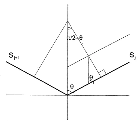
Let $s_{j}$ be the speed of $E_{j}$. Let $2\theta_{j}(0<\theta_{j}<\pi/2)$ be the angle between $S_{j}$
and $S_{j+1}$. Then we have
$s_{j}\sin\theta_{j}=k$.
The angle between $\nu_{j}$ and $|\nu_{j+1}-\nu_{j}|^{-1}(\nu_{j+1}-\nu_{j})\cross(\nu_{j}\cross\nu_{j+1})$ equals
Figure 7: The angle between surfaces $S_{j}$ and $S_{j+1}$
We get
$\sin\theta_{j}=\frac{\sqrt{\tau^{2}p_{j}^{2}+q_{j}^{2}}}{q_{j}\sqrt{1+\tau^{2}}}$
and thus
$s_{j}= \frac{cq_{j}}{\sqrt{\tau^{2}p_{j}^{2}+q_{j}^{2}}}$
.
The speed of $E_{j}$ toward the z-axis equals
$\frac{\sqrt{\tau^{2}p_{j}^{2}+q_{j}^{2}}}{q_{j}}s_{j}=k\sqrt{1+\tau^{2}}=c$
,
which coincides with the speed of $V$
.
Since weare
now using the movingcoordinate, this fact suggests that $E_{j}$ satisfies $\mathcal{L}(E_{j})=0$. We will check
this later. We use the following change of variables
where $R_{j}^{T}$ is the transposed matrix of $R_{j}$. Here we set
$R_{j} def=[0\frac{B_{j}-B_{j+1}}{q_{j}}\frac{A_{j}-A_{j+1}}{q_{j}}$ $\frac\frac{\tau(B_{j}-B_{j+1})p_{j}}{\tau(A_{j+1}-A_{j})p_{j},q\sqrt{\tau^{2}p_{j}^{2}+q_{j}^{2}}q_{j}\sqrt{\tau^{2}p_{j}^{2}+q_{j}^{2}}\frac{jq_{j}}{\sqrt{\tau^{2}p_{j}^{2}+q_{j}^{2}}}}$
$- \frac{\sqrt{}\tau^{2}p_{j}^{2}+q_{j}^{2}\sqrt A_{j+1}-A_{j}B_{j}-B_{j+1}\tau^{2}p_{j}^{2}+q_{j}^{2}\tau p_{j}}{\sqrt{\tau^{2}p_{j}^{2}+q_{j}^{2}}}\frac\frac 1$
and
$(R_{j})^{T}=( \frac{B_{j}-B_{j+1}}{\sqrt{\tau^{2}p_{j}^{2}+q_{j}^{2}}}\frac{\tau()p_{j}\frac{A_{j}-A_{j+1}}{B_{j}-B_{j+1}q_{j}}}{q_{j}\sqrt{\tau^{2}p_{j}^{2}+q_{j}^{2}}}$ $\frac{\tau(A_{j+1^{q_{j}}}-A_{j})p_{j}B_{j}-B_{j+1}}{q_{j}\sqrt{\tau^{2}p_{j}^{2}+q_{j}^{2}}}\frac{A_{j+1}-A_{j}}{\sqrt{\tau^{2}p_{j}^{2}+q_{j}^{2}}}$
$- \frac{\sqrt{}\tau^{2}p_{j}^{2}+q_{j}^{2}q_{j}\tau p_{j}0}{\sqrt{\tau^{2}p_{j}^{2}+q_{j}^{2}}}\frac$
$)$
Now we define $E_{j}$ as
$E_{j}(x, y, z) def=v_{*}(\frac{(A_{j}-A_{j+1})x+(B_{j}-B_{j+1})y}{q_{j}}$,
$\frac{\tau(B_{j}-B_{j+1})p_{j}x+\tau(A_{j+1}-A_{j})p_{j}y+q_{j}^{2}z}{q_{j}\sqrt{\tau^{2}p_{j}^{2}+q_{j}^{2}}}\rangle\frac{cq_{j}}{\sqrt{\tau^{2}p_{j}^{2}+q_{j}^{2}}})$
Then after calculations we obtain
$\mathcal{L}[E_{j}]=$
$-(v_{*})_{\zeta\xi}(\xi, \eta;s_{j})-(v_{*})_{\eta\eta}(\xi, \eta;s_{j})-s_{j}(v_{*})_{\eta}(\xi, \eta;s_{j})-f(v_{*}(\xi, \eta;s_{j}))=0$
in $\mathbb{R}^{3}$. Thus
for each $j(1\leq j\leq n)E_{j}(x)$ satisfies (3). We call $E_{j}$
a
planarV-form front associated with
an
edge $\Gamma_{j}$.We put
Then we have
$\mathbb{R}^{3}=\bigcup_{j=1}^{n}Q_{j}$.
We define
$\hat{E}(x)^{d}=^{ef}\max_{1\leq j\leq n}E_{j}(x)$
.
Since $E_{j}$ is strictly monotone decreasing in $z$ for each $j,\hat{E}$ is also strictly monotone decreasing in $z$. It satisfies
$\underline{v}(x)<\hat{E}(x)<V(x)$ $x\in \mathbb{R}^{3}$
and
$\lim_{\gammaarrow\infty}\sup_{x\in D(\gamma)}|\hat{E}(x)-\underline{v}(x)|=0$
.
(19)A pyramidal traveling front is uniquely determined
as
a combination oftwo-dimensional V-form fronts.
Corollary 4 ([22]) Let $h$ be as in (7) and let $V$ be the pyramidal traveling
wave
associated with $z=h(x, y)$, that is, $V$satisfies
(3) and (9).If
(3)has a solution $v$ with
$\lim_{Rarrow\infty}\sup_{|x|\geq R}|v(x)-\hat{E}(x)|=0$,
then one has $v\equiv V$.
Thus
a
three-dimensional travelingwave
is uniquely determinedas
a
combination of two-dimensional V-form waves.
References
[1] D. G. Aronson and H. F. Weinberger, Nonlinear diffusion in
popula-tion genetics, Partial Differential Equations and Related Topics, ed.
J. A. Goldstein, Lecture Notes in Mathematics,
446
(1975)5-49.
[2] X. Chen, Existence, uniqueness, and asymptotic stability of traveling
waves
in nonlocal evolution equations, Adv. Differential Equations, 2,[3] X. Chen, J-S. Guo, F. Hamel, H. Ninomiya and J-M Roquejoffre,
Tkaveling waves with paraboloid like interfaces for balanced bistable
dynamics, Ann. I. H. Poincar\’e, AN 24, (2007) 369-393.
[4] P.
C.
Fife and J. B. McLeod, The approach of solutionsof
nonlin-ear diffusion equations to travelling bont solutions, Arch. Rat. Mech.
Anal., 65 (1977) 335-361.
[5] D. Gilbarg and N.S. Trudinger, Elliptic Partial Differential Equations
of Second Order, Springer-Verlag, Berlin,
1983.
[6] F. Hamel, R. Monneau and J.-M. Roquejoffie, Stability of travelling
waves in a model for conical flames in two space dimensions, Ann.
Scient. Ec. Norm. Sup. 4\‘eme s\’erie,
t.37
(2004) 469-506.[7] F. Hamel, R. Monneau and J.-M. Roquejoffre, Existence and
quali-tative properties of multidimensional conical bistable fronts, Discrete
Contin. Dyn. Syst., 13, No. 4 (2005) 1069-1096.
[8] F. Hamel, R. Monneau and J.-M. Roquejoffre, Asymptotic properties
and classification of bistable fronts with Lipschitz level sets, Discrete
Contin. Dyn. Syst., 14, No. 1 (2006) 75-92.
[9] Y. I. Kanel’, Certain problems
on
equations in the theory of burning,Soviet. Math. Dokl., 2, (1961)
48-51.
[10] Y. I. Kanel’, Stabilization ofsolutions of the Cauchy problemfor
equa-tions encountered in combustion theory, Mat. Sb. (N.S.), 59 (101)
(1962) 245-288.
[11] F. Hamel and N. Nadirashvili, TYavelling fronts and entire solutions of
the Fisher-KPP equation in $\mathbb{R}^{N}$, Arch. Rat. Mech. Anal., 157, (2001)
91-163.
[12] M. Haragus, A. Scheel, Corner defects in almost planar interface
prop-agation, Ann. I. H. Poincar\’e, AN 23 (2006)
283-329.
[13] C. D. Levermore and J. X. Xin, Multidimensional stabilityoftraveling
waves
in a bistable reaction-diffusion equation II, Comm. Par. Diff.[14] T. Kapitula, Multidimensional stability of planar traveling waves,
Trans. Amer. Math. Soc.,
349
(1997)257-269.
[15] H. Matano, M. Nara and M. Taniguchi, Stability of planar waves in
the Allen-Cahn equation, preprint
[16] J. Nagumo, S. Yoshizawa and S. Arimoto, Bistable transmission lines,
IEEE ‘llrans. Circuit Theory, CT-12, No 3 (1965) 400-412.
[17] H. Ninomiya and M. Taniguchi, Existence and global stability of
trav-eling curved fronts in the Allen-Cahn equations, J. Differential
Equa-tions, 213, No 1 (2005) 204-233.
[18] H. Ninomiya and M. Taniguchi, Global stability of traveling curved
fronts in the Allen-Cahn equations, Discrete Contin. Dyn. Syst., 15,
No 3 (2006) 819-832.
[19] M. H. Protter and H. F. Weinberger, Maximum Principles in
Differ-ential Equations, Springer-Verlag, Berlin, 1984.
[20] D. H. Sattinger, Monotone methods in nonlinearelliptic and parabolic
boundary value problems, Indiana Univ. Math. J., 21, No 11 (1972)
979-1000.
[21] M. Taniguchi, baveling fronts of pyramidal shapes in the $Allenarrow$Cahn
equations, SIAM J. Math. Anal., 39, No 1 (2007) 319-344.
[22] M. Taniguchi, The uniqueness and asymptotic stability of pyramidal
traveling fronts in the Allen-Cahn equations, J. Differential Equations
(accepted for publication)
[23] J. X. Xin, Multidimensional stability of traveling waves in a bistable
reaction-diffusion equation I, Comm. Par. Diff. Eq., 17 (1992)

![Figure 4: Contour lines of a two-dimensional V-form wave $v_{*}(x,y)$ ([17]).](https://thumb-ap.123doks.com/thumbv2/123deta/5986264.1060249/9.892.292.616.146.479/figure-contour-lines-dimensional-v-form-wave-v.webp)