VISCOUS SHOCK PROFILES FOR 2×2 SYSTEMS OF HYPERBOLIC CONSERVATION LAWS WITH QUADRATIC FLUX FUNCTIONS (Mathematical Analysis in Fluid and Gas Dynamics)

(1)

VISCOUS

SHOCK

PROFILES

FOR

2\times 2

SYSTEMS

OF

HYPERBOLIC

CONSERVATION

LAWS

WITH

QUADRATIC

FLUX FUNCTIONS

大阪電気通信大学・工学部浅倉史興 (FUMIOKI ASAKURA)

OSAKA ELECTRO-COMMUNICATION UNIV.

[email protected]

国際基督教大学・教養学部山崎満 (MITSURU YAMAZAKI)

INTERNATIONAL CHRISTIAN UNIV.

[email protected]

1. INTRODUCTION

The purpose of this paper is to understand the shock

wave

structure of conservation

laws that

come

from the extraction of petroleum.

An oil reservoir is a subsurface pool of hydrocarbons contained in porous rock

foririations. If the underground pressure of in the reservoir is sufficient, tlien the oil is

naturally

forced

to the surface and extracted by valves on the well. This is called the

primary recovery and usually about 20% of the oil in a oil reservoir can be extracted.

Over the lifetime ofthe well, the underground pressure will be insufficient to force

the oil to the surface. Secondary

recovew

techniques increase the reservoir pressure by

injecting water and gas (air

or

CO2). Generally 25% to 35% of the oil in

a

oil reservoir

can

be extracted by primary and secondary recovery together.

OilProducer

(2)

Water-Alternating-Gas (WAG) Enhanced Oil Recovery: Although the watcr

injection $\}_{1’\ }$ good sweep cfficiericy, 40 to $60^{(}f_{(}/$ of the original oil on-site is left behind

at the end of the injection. The

gas

injection has good displacement eff\’iciency but is

an

expensive operation. Hence the injection of

gas

after water followed by water and

gas injection

causes

significant redistribution of fluids in the reservoir and will be more

efficient than injection of water

or

gag alone.

Because of the gravity, three $I$)

$\}_{1d6}es^{\backslash }$: oil, gas and water

are

separated frorii

one

another away from the WAG injector and it is only

near

the injector where three phase

flow actually

occurs.

Mathernatical structure of the three phase flows has been

inves-tigated by many authors (for example, Marchesin-Plohr [7], Medeiros [8],

Schaeffer-Shearer [10]$)$ and, in this paper,

we

shall confine ourselves particularly to their shock

wave structure.

Stone’s

Model: Ill order to simplify $t1_{1}etfiree- p1_{1R}e$ flow in

a

porous medium,

we

neglect the gr\‘avity and

assume

that the inedium is homogeneous and the flow is

in-compressible and immiscible. Let us denote:

water gas oil

Volume Fractioiis: $S\eta r$ ニ $u$ _{$s_{G}=v$} $so=1-u-\prime u$

Permeability Functions: んw んG $k_{O}$

Fluid Viscosity: $\mu_{W}$ $\mu_{G}$ $\mu_{O}$

Fluid Velocity: $v_{W}-$ $v_{G}$ $\uparrow)0$

Pressure: $p_{W}$ $p_{G}$ $p_{O}$

The relationship betweenthe flow rate and the pressure gradient isexpresse$(1$ by Darcy’.s

Law

$v_{i}=- \frac{k_{i}}{\mu_{i}}\nabla p_{i}$, $i=W,$$G,$$O$.

It is usually assumed tbat the water and gas permeability functions depend only

on

the water \‘and gas volume fraction

$k_{W}=k_{W}(u)$, $k_{G}=k_{G}(v)$

which is called Stone’s assumption. We finally $a_{\iota}ssume$ that the flow is

one

dimensional

and the capillary pressure is negligible.

By using relative permeability

_functions

$f(u)= \frac{k_{W}(u)}{\mu_{l}w}$, $g(v)= \frac{k_{G}(v)}{\mu_{G}}$ $h(u, v)= \frac{k_{O}(u,v)}{\mu_{W}}$

the mass conservation laws

are

expressed in the form

Water: $\frac{\partial’u}{\partial t}+\frac{\partial’}{\partial x}[\frac{f(u)}{f(u)+g(v)+h(u,v)}]$ $=$ $0$, (1)

(3)

in $\Omega$ :

$0<u+v<1,$

$u,$ $t)>0$ ([7],[8], [10]). These equations constitute

a

system of

conservation laws that is discussed in this paper.

Hyperbolicity: We say that the system of equations (1) and (2) is hyperbolic, when

tlie Jacobian matrix of tfie flux function has real eigenvalues $\lambda_{1}(U),$ $\lambda_{2}(U)$ for any $U\in$

$\zeta)$. If, in particular, tfiese eigenvalues

are

distinct: $\lambda_{1}(U)<\lambda_{2}(U)$, the system is calle$(1$

strictly hyperbolic at $U$. Corresponding right eigenvectors

are

denoted by _{$R_{1}(U),$ $R_{2}(U)$}

respectively. A state $U^{*}\in\Omega$ is called an umbilic point, if _{$\lambda_{1}(U^{*})=\lambda_{2}(U^{*})$} _and

the Jacobian matrix is diagonalizable, hence a scalar matrix. Marchesin, Paes-Leme,

Schaeffer and Shearer have shown in [10].

Theorem 1 (Existence of Umbilic Point) Assume that

$h(u, v)=h(1-u-v)$

and

$f(O)=g(O)=h(O)=0,$ $f”(u),$$g”(v),$ $h”(w)>0$

.

Then the system

of

_{equations (1), (2)}

is hyperbolic and has a unique urnbilic point in $\zeta l$.

After the change of unknown functions, we may

assume

that $U^{*}=O$ and _{$F(O)=O$ .}

$T\}ius$

we

fiave the Taylor expansion of the flux function _$F(U)$ near _$U=O$_:

$F(U)=\lambda^{*}U+Q(U)+O(1)|U|^{3}$

where $\lambda^{*}=\lambda_{1}(U^{*})=\lambda_{2}(U^{*})$ and $Q$ : $R^{2}arrow R^{2}$ is a homogeneous quadratic mapping.

After the Galilean change of variables: $xarrow x-\lambda^{*}t$, we observe that the system of

equations (1) and (2) is reduced to

$U_{t}+Q(U)_{x}=O$, $(x_{t}t)\in R\cross R_{+}$,

modulo Iligfier order terrns. By

a

_{cliange of unknown fuiictions} $V=S^{-1}U$ _with

_a

regular constant matrix $S$,

we

have

a new

system of equations _{$V_{f}+P(V)_{x}=0$} with

$P(V)=S^{-1}Q(SV)$ . Hence we say that two quadratic mappings $Q_{1}(U)$ and $Q_{2}(U)$

are

equivalent, if there is

a

constant matrix $S\in GL_{2}(R)$ such

$Q_{2}(U)=S^{-1}Q_{1}(SU)$ for all $U\in R^{2}$.

Scliaeffer-Shearer

[10] shows that every hyperbolic quadratic mapping $Q(U)$ with

an

isolated umbilic point $U=O$ is equivalent to

$Q(U)= \frac{1}{2}(\begin{array}{l}au^{2}+2buv+v^{2}bu^{2}+2u^{r}\{j\end{array})=\frac{1}{2}\nabla C(U)$, (3)

$C(U)= \frac{1}{3}au^{3}+bu^{2}v+uv^{2}$. (4)

wfiere $a$ and $b$

are

two real parameters satisfying _{$a\neq 1+b^{2}$}. For Stone’s model, either

Case I: $a< \frac{3}{4}b^{2}$ or Case II: _{$\frac{3}{4}b^{2}<a<1+b^{2}’$}

.

A constant characteristic vector field $\Xi={}^{t}(1,$$\xi)$ exists if and only if

$\xi^{3’}+2b\xi^{2}+(a-2)\xi-b=-\Xi^{\perp}\nabla Q(\Xi)\Xi=0$

Three district (real) roots

are

denoted by $\mu_{1},$$\mu_{2},$ $\mu_{3}$ and Medians

are

defined by $\Lambda l_{j}$ :

(4)

Gomes’ Paper [4] and

our

aim: M. E. S. Gomcs has proved the existence of

viscous

shock profiles for shock

waves

in

Case

I by topological metliods and also sliowii

an

exarnple of compressive shock

wave

without viscous shock profiles. The airn of this

paper is to complete her results by using both topological and analytical methods:

existence ofviscous profiles in

Case

I and II and general condition for non-existence of

viscous profiles. We shall show in this paper only outline of proof and details will be

published in Asakura-Yarnazaki [2].

2. UNDERCOMPRESSIVE

AND

OVERCOMPRESSIVE

SHOCK

WAVES

Rankine-Hugoniot condition: A jump discontinuity defined by

$U(x, t)=\{\begin{array}{l}U_{L} for x<st,U_{R} for x>st,\end{array}$ (5)

with a real constant $s$, is a piecewise constant weak solution to the the conservation

laws (3), if and only if these quantities satisfy the Ranんine-Hugoniot condition:

$s(U_{R}-U_{L})=Q(U_{R})-Q(U_{L})$. (6)

The weak solution (5) satisfying (6) is often called a shock wave of speed $s$ joining the

state $U_{L}$,

on

the left, to the state $U_{R}$,

on

the right.

Compressive shock

wave:

The shock

wave

is said to be a j-compressive $(j=1,2)$

if tfie speed satisfies the Lax entropy conditions:

$\lambda_{j}(U_{R})<6<\lambda_{j}(U_{L}),$ $\lambda_{j-1}(U_{L})<s<\lambda_{j+1}(U_{R})$

Here

we

adopt the convention $\lambda_{0}=-\infty$ and $\lambda_{3}=\infty$.

l-compressive $2- com\rho ressive$

(5)

Undercompressive shock

wave:

Undercompressive if $\sigma$

.

satisfies

$\lambda_{1}(U_{R})<_{(6^{\text{・}}}<\lambda_{2}(U_{R}),$ $\lambda_{1}(U_{L})<_{\iota}s<\lambda_{2}(U_{L})$

Undercompressive

$Fi_{b^{111(}’\backslash }3:\iota\dagger_{11t}1Y..Jt.,|\zeta_{)}^{t}$ _wi$\iota ve$

Overcompressive shock

wave:

Overcompressive if.$s$ satisfies

$\lambda_{1}(U_{R})<s<\lambda_{1}(U_{L}),$ $\lambda_{2}(U_{R})<s<\lambda_{2}(U_{L})$

Overcompressive

(6)

Stability and Admissibility of Shock Waves: It is generally believed

$\bullet$ Compressive shock

waves are

generally stable and admissibility is independent of

diffusion matrices in a generic class.

$\bullet$ Undercompressive shock

waves are

stable with additional (kinetic) $con(lition$ and

admissibility depends

on

diffusion matrices.

$\bullet$ Overcompressive shock

waves are

generally unstable.

Admissibility is defined in next section.

3. VISCOUS

SHOCK

PROFILES

Admissibility: The jump discontinuity is said to be admissible if $tIiere$ exists a

travelling

wave

solution $U_{\epsilon}(x, t)= \hat{U}(\frac{x-st}{\epsilon})$ to $tI_{1}e$ parabolic systeni

$U_{t}+Q(U)_{x}=\epsilon U_{x}$

丁’

$\epsilon>0$ (7)

satisfyirig $U_{\epsilon}(+\infty, t)=U_{R},$ $U_{\epsilon}(-\infty, t)=U_{L}$. Tlie vector fuiiction $\hat{U}=\hat{U}(\xi)$ is called a

viscous shock $prof\dot{\ddagger}le$.

Differential Equations and Vector Field: By integrating (7), $\hat{U}(\xi)$ satisfies

a

system of nonlinear differential equations

$\frac{d\hat{U}}{d\xi}$

$=$ $-6^{\backslash }(\hat{U}-U_{L})+F(\hat{U})-F(U_{L})$ $=$ $X_{s}(U, U_{L})$

Note that $U_{L}$ is a critical point of $X_{s}(U, U_{L})$ and by Rankine-Hugoniot condition $U_{R}$

is also a critical point. Since the flux functions has

a

potential $C(U)$_, by setting

$\phi_{s}(U_{L}, U)=C(U)-\nabla C(U_{L})\cdot(U-U_{L})-s|U-U_{L}|^{2}$,

the differential equations turn out to be

$\frac{d\hat{U}}{d\xi}=\frac{1}{2}\nabla\phi_{\theta}(U_{L},\hat{U})$

.

(8)

Hence the adinissibility is equivalent to the existence of solution of this equations

satisfying tfie boundary conditions at infinity:

$\lim_{\xiarrow-\infty}\hat{U}(\xi)=U_{L},\lim_{\xiarrow\infty}\hat{U}(\xi)=U_{R}$

orto finding flow connectingtwo criticalpoints $U_{L}$ and $U_{R}$ of the vector field $\nabla\phi_{s}(U_{L}, U)$

(7)

4. EXISTENCE

OF

VISCOUS

SHOCK PROFILES

Critical Points: Classification of compressive, undercompressive and

overcompres-sive shock

waves

corresponds to that of critical points:

There

are

at most four critical points in the finite plane (intersection of two conics).

In

four

critical point

case:

Case

I:

one

node and three saddles [4], $C$_\‘ase II: two nodes and two saddles [1]

Saddle-Saddle Connection: Flow of a saddle-saddle connection lies on $M_{j},$ $j=$

$1,2,3$ ([3],[4]). If $U_{L}\in\Lambda jf_{j’},$ $j=1,2,3$, The equation of viscous shock profile turns out

to be the Burgers equation

$\frac{du}{d\xi}=\frac{b+2\mu_{j}}{2\mu_{j}}(u-u_{1})(u-u_{L}),$ $u_{1}=-u_{L}+ \frac{2\mu_{j}}{b+2\mu_{j}}s$.

By direct computations

we

have

Theoreni 2 ([2]) Undereompressive shock.$\sigma$ with viscous profile exist only

on

$M_{1}\cup$

$M_{2}’\cup M_{3}$ in Case $I$ $ar\iota d$ on $\Lambda l_{1}\cup A/l_{3}$ in Case $\Pi$. Overcornp$\gamma\cdot e66^{\prime ive}$ shocks with viscous

profile exist only on $M_{2}$ in Case $\Pi$.

Existence of Viscous Profiles: If there

are no

saddle-saddle connection, the

con-nection problem is settled

as

the following:

Theorem 3 ([2], Case I)

_If

$U_{L}$ is a node, then

for

each single saddle point there

exists a viscous shock profile between $U_{L}$ and the saddle point.

Theorem 4 ([2], Case II) Two nodes consist

_of

one

attractor and one repeller.

_If

$U_{L}$ is

a

node, then

for

each

of

two saddle points, there exists

a

viscous shock profile

shock profile between $U_{L}$ and the saddle point. Moreover there exist infinitely many

viscous shock profiles

_from

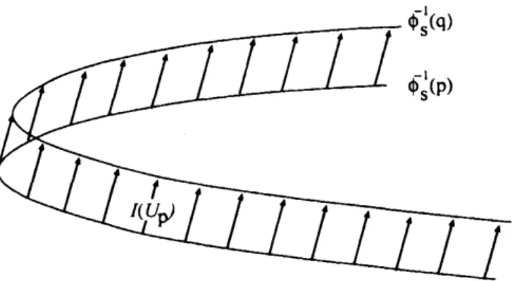
the repeller to the attractor.

Proof of the above both theorems is based

on

a generalization of the first theorem of

Morse to non-compact level sets: if $|\nabla\phi_{s}(U, U_{L})|^{2}\geq m$ for any $U\in\phi_{s}^{-1}[p, q]$, then

(8)

$Fi_{h)}\backslash .\backslash AI_{(1\backslash (}|\backslash$ Foliation

where $I(U_{\rho})$ : integral

curves

of the equation (8) connecting $U_{p}\in\phi_{8}^{-1}(p)$ and

a

certain

point on the level set $\phi_{n}^{-1}(q)$.

Case I: We inay

assume

tliat $U_{L}$ is a repeller. Figure 7 to 9 show nine level

curves

of $\phi_{s}$ for $a=0.5,$$b=1,$ $s=-3.5$ and $U_{L}=\ell(1,1)$. Let $\epsilon$ be

a

positive small constant.

$T1_{1}e$ level set $\{\phi_{s}=\epsilon\}$ is composed of

a

small closed curve enclosing $U_{L}$ and three

unbounded regular

curves

$($Fig 7: $\phi_{\theta}=10.00)$. Suppose that

a

critical point $U_{1}$ exists

on

the level set $\{\phi_{s}(U)=p_{1}\}$, $($Fig.7: $p_{1}=25.88)$ such that there is

no

critical point

in $\{\epsilon\leq\phi_{s}(U)\leq p_{1}-\epsilon\}$. By the Morse lemma, we find that $\phi_{s}^{-1}[\epsilon,p_{1}-\epsilon]$ is a Morse

foliation. When the level

curve

meets

a

critical point for $\phi_{s}(U)=p_{1}$,

an

integral

curve

connects two critical points $($Fig.7: $\phi,$ $=25.88)$. Repeating this argument, we have

three trajectories connecting critical points (Fig 8, 9).

Figure 6: Flow af a $C_{/I}^{1}\cdot itit_{f}\iota 1$ Poiiit

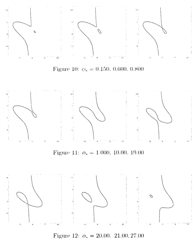
Case II: We may

assume

that $U_{L}$ is

a

repeller. Figure 10 to 12 show nine level

curves

of $\phi_{s}$ for $a=1.5,$ $b=1,$ $s=-1$ and $U_{L}={}^{t}(1,1)$

.

The level set

{

$\phi_{s}=\epsilon$ :

small}

is composed of a small closed

curve

enclosing $U_{L}$ and a single unbounded regular

curves

in this

case

$($Fig 10: $\phi_{s}=0.150)$. Suppose that the first critical point $U_{1}$

exists

on

$t\}_{1}e$ level set _{$\{\phi_{R}(U)=p_{1}\}$}, $($Fig.10: $p_{1}=0.800)$ such that there is

no

critical point in $\{\epsilon\leq\phi_{s}(U)\leq p_{1}-\epsilon\}$

.

By the

same

argument

as

above,

we

find a

trajectory connecting $U_{L}$ and the first critical point $($Fig 10: $\phi_{s}=0.800)$. Repeating

(9)

Above the second critical point,

we

have

a

closed

curve

and

a

single unbounded

curve

(Fig 12: $\phi_{s}=21.00$, 27.00).

Since

the closed

curve

encloses

an

attractor, we conclude

that there

are

infinitely many trajectories issuingfrom $U_{L}$ and drawn into the attractor.

Figure 7: $c/’)_{\backslash }$. $=1(].(\}(). 23.()(). 2_{\iota}^{\ulcorner}).88$

$\lrcorner 0^{--}\overline{v}^{-}$

$-$

$\lrcorner 0|$ $\aleph$

$|$

$0$

Figure 8: $(/’J.\backslash =\backslash \sigma).()().()_{t}^{\ulcorner}).()()$. $8_{l})_{t}).)$

(10)

$\ovalbox{\tt\small REJECT}_{10}\ovalbox{\tt\small REJECT}$

Figure 10: $c_{l})_{\backslash }=|).1_{\iota}\ulcorner)()$. $().()()()$. $().b()()$

1$(|\mathfrak{l}$ 10 $1$ $|$ $|$ $r$ $\mathfrak{l}.|$ $\iota$ $1$ $1$ $r$ $tt$ $|\ulcorner$ $t$

.

$Fi_{h^{tt1(}}\cdot\backslash 11:\zeta^{}).,$ $=1.()()(|. 1().()(). 1^{(}).()()$ 1$||$ $|$.

..

$d|$ $1$ $|$ $\uparrow t$’ $1111$

..

$\Im$ $)(t$ .,. $\overline{1(}$ $Fi_{\epsilon}(;1t1^{\cdot}(112:(|)_{\tau}=2().()(). 21.t)(I,$$27.()(|$

5. COMPRESSIVE SHOCK

WITHOUT

VISCOUS SHOCK

PROFILE

Liu-Oleinik Condition: Let

us

denote: $\mathcal{H}(U_{L})$ : $U=U(\xi;U_{L})$ the Hugoniot curve

issuing from $U_{L};s(\xi)$ : the shock speed at $U(\xi);U_{R}=U(\xi_{1})$

.

We say that $U_{L}$ and $U_{R}$

satisfy tlie (strict) $Liu- Oleir\iota ik$ condition if $s(\xi_{1})<s(\zeta)$ for all $0\leq\xi<\xi_{1}$ ([9]).

For strictly hyperbolic systems,

as

long as $U_{R}$ is sufficiently close to $U_{L}$, there exists

a

viscous shock profile connecting these states ifand only ifthey satisfy the Liu-Oleinik

(11)

$Figltl\cdot(|$ $L$3: $]_{\lrcorner}i_{1}\iota-()1\epsilon i_{11}ik\zeta^{1}oii(1itioi1$

State $U_{L}$

on a

Median (Case I): In this case, the Hugoniot

curves

are composed

of the median and a hyperbola, and their intersection points

are

$U_{L}$(first bifurcation

poiIit) and $U_{*}$ (secon(1 bifurcation poirit). We

can

deduce by TheoreIn 2 that tliere is

a saddle-saddle connection (Fig. 14: left).

Theorern 5 ([2]) Suppose that the medians and the

_inflection

curves inter.sect only at

the origin $O$ and that _{$U_{L}\in M_{j}\backslash \{O\}.(j=1,2,3)$}. Then $tf\iota er\cdot e$ exists one branch $\mathcal{H}_{*}$

of

the hyperbola $\mathcal{H}_{j}(U_{L})$ issuing _{$fro7nU_{*}$} such that the state $U_{L}$, on the left, can be joined

to any $state\in \mathcal{H}_{*}$ sufficiently close to $U_{*}$,

on

the right, by

an

inadmissible, compressive

Liu-Oleinik shock. In this case, there exists

a saddle-saddle

connection along $M_{j}$.

Outline of proof: Let $U_{L}\in M_{1}$ and $u_{L}>0$

.

We find by direct computation that the

2-shock

curve

issuing frorn $U_{L}$ is composed ofthe segment $\overline{U_{L}U_{*}}$ and

one

branch of the

hyperbola $\mathcal{H}_{j}$ issuing from $U_{*}$

.

Figure 14: Hugoniot $I_{J((11b\dot{c}\mathfrak{l}11(1^{\zeta_{)}^{t}}1_{1t(}\cdot]^{\zeta_{)}^{\tau}}\backslash }vI\backslash ^{r}\llcorner 1)1^{t}((1$

Since $\sigma\cdot=\lambda_{2}$ and $\dot{s}\neq\dot{\lambda}_{2}$ at $U_{*}$, one branch of hyperbola containing $U_{*}$ is

a

com-pressive branch ofthe 2-shock

curve.

Hence by choosing the shock speed $s$ close to $s_{*}$

we

have

a

2-cornpressive shock conriecting $U_{L}$ and

a

st\‘ate $U_{R}$ that is close to $U_{*}$

. As we

(12)

which is close to $U_{*}$, hence close to $U_{R}$. Thus

we

conclude from the configuration of

trajectories tliat it is impossible.

Figure 14 is the Hugoniot

curves

and the graph of shock speed for $a=0.1$,

$b=1,$ $U_{L}={}^{t}(0.5,0.5\mu_{1}),$ _{$\mu_{1}=-2.65004,$ $\mu_{2}=-0.369954,$} $\mu_{3}=1.02,$ $U_{*}=$

${}^{t}(-0.0484773$,0.128465$)$, $s_{*}=0.653999$; the par\‘ameter of the shock speed is $\xi=\underline{v}\underline{-}v$ $u-u_{\iota}$

.

In the graph of shock speed, $s$ decreases from $\lambda_{2}(U_{L})$ to $\lambda_{*}$ along _{$\xi=\mu_{1}$}

.

then the

compressive blanch goes to the right. It is clear from this figure, the Liu-Oleinik

con-dition actually holds. Figure 15 shows the level

curves

of the potential function for

「$\overline{\prime\prime}|i|$ $r$ _{$\prime’’-\neg$} $\text{ノ^{}\prime}$ $arrow–\cdot\cdot’-\cdot\simarrow\sim\cdots-\cdot--$ $arrow..-\cdot\sim-\cdot-\cdots\cdot,\ldots\ldots-$ $|$ ’

$L–$

$\text{沖_{}-\vee\cdot-arrow-}\rfloor$

Figure $1_{\backslash )}^{\ulcorner}:\backslash \cdot=().r)4C),$ $\phi\backslash \backslash =(\}.47_{\backslash }^{\cdot}\backslash ()78_{t}^{r_{J}}$ (left):

$\phi_{l},$ $=(I.47’)()8()$ (riglit)

$s=0,646$. The left figure: $\phi_{s}=0.4730785$ shows the connection of $U_{L}$ and

a

certain

state

on

the median $M_{1}$, hence the existence of

an

undercompressive shock

wave.

The

right one shows a small closed level

curve

that encloses

an

attractor.

References

[1] Asakura F.

&Yamazaki

M. (2005) Geometry of Hugoniot

curves

in $2\cross 2$ systems of

hyperbolic conservation laws with quadratic flux functions, IMA J. Appl. Math.,

70, no. 6, 700-722.

[2] Asakura F.

&Yamazaki

M. (2008) Viscous Shock Profiles for 2 $\cross 2$ Systems of

hyperbolic conservation laws with

an

umbilic point, to appear J. Hyperbolic

Dif-ferential Equations.

[3] Chicone C. (1979) Quadratic gradients on the plane

are

generically Morse-Smale,

J. Differential Equations, 33, 159-166.

[4]

Gonies

M. E.

S.

(1989) Riemann problems requiring

a

viscous profile eritropy

condition, Adv. Appl. Math., 10, 285-323.

$|^{r_{)}}]$ Liu T.-P. (1975b) The Riemann problem for general systems of conserv\‘ation laws.

(13)

[6] Majda A.

&Pego

R. (1985) Stable Viscosity

Matrices

fo Systems of

Conservation

Laws, J. Differential Equations, 56, 229-262.

[7] Marchesin D.

&Plohr

B. (2001) Theory _{of Three-Phase Flow Applied to}

Water-Alternating-Gas Enhanced Oil Recovery, Hyperbolic Problems; Theory, Numerics,

Applications, Vol.II, Birkh\"auser Verlag,

693-702.

[8] Medeiros H. B. (1992) Stable Hyperbolic Singularities for Three-Pha.ge _Flow

Mod-els in Oil Reservoir Simulation, Acta Applicandae Mathematicae, 28, 135-159.

$[^{(})]$ Oleinik $0$

.

(1957) Discontinuous solutions of non-linear differential

equations,

Amer.

Math. Soc. Transl. Ser. 2,

26

(1957),

95-172.

[1()] Schaeffer D.

&Shearer

M. (1987) The $c1\ ;_{t};ification$ of$2\cross 2$ systems ofnon-strictly

hyperbolic conservation laws, with applications to oil recovery, Comm. Pure Appl.