On the relation between Borel sum and classical solution for Cauchy problem of Airy's and Beam's PDE (Deformation of differential equations and asymptotic analysis)

On

the relation between Borel

sum

and

classical solution for

Cauchy problem

of

Airy’s

and

Beam’s PDE

Kunio Ichinobe

(市延

邦夫

)

Graduate

School

of

Mathematics,

Nagoya

University

( 多元数理科学研究科,

名古屋大学

)

1

Introduction

We consider the following two Cauchy problems for partial differential equations of

non-Kowalevski type

$(\mathrm{A})_{\mathrm{R}}$ $\partial_{t}u(t, x)=\partial_{x}^{3}u(t, x)$, $u(0, x)=\varphi(x)$, $(t>0, x\in \mathbb{R})$

$(\mathrm{B})_{\mathrm{R}}$ $\partial_{t}u(t, x)=-\partial_{x}^{4}u(t, x)$, $u(0, x)=\varphi(x)$, $(t >0, x\in \mathbb{R})$

where the equation $(\mathrm{A})_{\mathrm{R}}$ is called the “Airy equation” and the equation $(\mathrm{B})_{\mathrm{R}}$ is called

the “Beam equation” , respectively.

The purpose in this note is to give the relationship between the “Classical solution”

and the “Borel sum” of each Cauchy problem in complex $\mathbb{C}^{2}$ plane. Precisely,

we

shall

show that the Classical solution ofthe Cauchy problem is derived from adeformation of

path ofintegration of the Borel

sum

in 0direction under

some

conditions for the Cauchy

data.

We state the contents of the following sections. In Section2we shallgive the “Classical

solution”. In Section 3we shall give the definition of Borel summability, known results

and the “Borel sum”. In Section 4our Claim which gives the relationship between the

Borel sum and the Classical solution will be stated and their proofs will be given. In

Section 5we shall give the sketch ofproofof Proposition 3.4

on

the kernel function of the

Borel sum. In Section 6we shallgive ageneralization ofour Claim as atheorem without

proof, which will be given in aforthcoming paper.

2Classical solution

Firstly,

we

shall give the “Classical solution”.

数理解析研究所講究録 1296 巻 2002 年 48-62

When we consider the Classical solution, we always

assume

that $t>0$, $x\in \mathbb{R}$ and for

the Cauchy data $\varphi\in S$, the rapidly decreasingfunctions inSchwartz’ sense, for simplicity.

Then it is known that the Cauchy problem $(\mathrm{A})_{\mathbb{R}}$ is uniquely solvable in $S$ and the solution

is given by

(2.1) $u_{c}^{A}(t, x)= \frac{1}{(3t)^{1/3}}\int_{-\infty}^{\infty}\varphi(x+y)Ai(\frac{y}{(3t)^{1/3}})dy$, $t$ $>0$, $x\in \mathrm{R}$.

Here $Ai$ denotes the Airy function which is defined by the following Airy’s integral

(2.2) $Ai(z)= \frac{1}{2\pi i}\int_{\gamma}\exp(zs-\frac{s^{3}}{3})ds$, $z\in \mathbb{C}$,

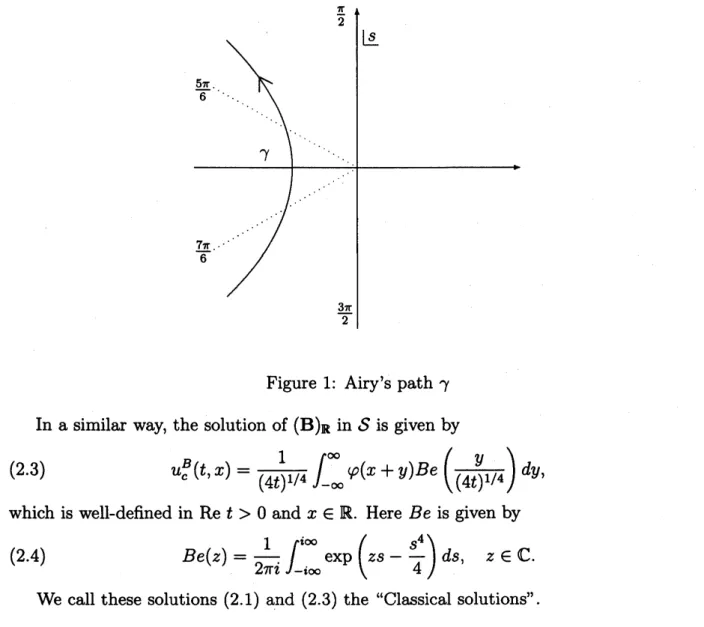
where the path $\gamma$ is any

curve

which begins at infinity in the sector $7\pi/6<\arg z<3\pi/2$

and ends at infinity in the sector $\pi/2<\arg z<5\pi/6$

.

(see Figure 1below)

Figure 1: Airy’s _{path 7} In asimilar way, the solution of $(\mathrm{B})_{\mathrm{R}}$ in $S$ is given by

(2.3) $u_{c}^{B}(t, x)= \frac{1}{(4t)^{1/4}}\int_{-\infty}^{\infty}\varphi(x+y)Be(\frac{y}{(4t)^{1/4}})dy$,

which is well-defined in ${\rm Re} t$ $>0$ and $x\in \mathbb{R}$. Here Be is given by

(2.4) Be(s) $= \frac{1}{2\pi i}\int_{-\dot{l}\infty}^{\dot{l}\infty}\exp(zs-\frac{s^{4}}{4})ds$, $z\in \mathbb{C}$. We call these solutions (2.1) and (2.3) the “Classical solutions”

3Borel

sum

Next,

we

shall give the “Borel sum” Precisely,

we

shall give the Borel

sums

of divergent solutions ofthe Cauchy problems $(\mathrm{A})_{\mathbb{C}}$and $(\mathrm{B})_{\mathbb{C}}$ whichare obtained from $(\mathrm{A})_{\mathbb{R}}$ and $(\mathrm{B})_{\mathbb{R}}$

by changing the real variables into the complex variables.

In order to do so, we consider the following Cauchy problem for partial differential

equations, which generalizes the Airy and the Beam equations.

$(\mathrm{C}\mathrm{P})_{\mathbb{C}}$ $\partial_{\tau}u(\tau, z)=\alpha\partial_{z}^{q}u(\tau, z)$, $u(0, z)=\varphi(z)$,

where $(\tau, z)\in \mathbb{C}^{2}$, $q\geq 2$, $\alpha\in \mathbb{C}\backslash \{0\}$ and the Cauchy data

$\varphi$is assumed to beholomorphic

in aneighbourhood of the origin.

This Cauchy problem $(\mathrm{C}\mathrm{P})_{\mathbb{C}}$ has aunique formal solution

(3.1) \^u$( \tau, z)=\sum_{n\geq 0}\alpha^{n}\varphi^{(qn)}(z)\frac{\tau^{n}}{n!}=\mathrm{p}\mathrm{u}\mathrm{t}$$\sum$ $u_{n}(z)\tau^{n}$.

By Cauchy’s integral formula,

we can

see that the coefficients $u_{n}(z)$ have the following

estimates: Thereexist positiveconstants $C$and $K$ for afixed$r>0$ such that the following

estimates hold

(3.2) $\max|z|\leq r|u_{n}(z)|\leq CK^{n}((q-1)n)!$, $n=0,1,2$,$\ldots$

.

By the assumption $q\geq 2$, the formal solution \^u$(\tau, z)$ is divergent. Precisely, the formal

solution \^u$(\tau, z)$ is called the formal power series of Gevrey order $(q-1)$ in $\tau$ variable.

We shall study the Borel summability of the divergent solution and we shall give the

Borel sum of the divergent solution.

Before stating the results, let us prepare some notations and definitions (cf. [Bal]).

3,1

_Notations

_and

_Definitions

1. Sector. For d $\in \mathbb{R}$, _$\beta>0$ and _{$\rho(0<\rho\leq\infty)$}, we define asector _{$5(\mathrm{d}, \beta, \rho)$} by

(3.3) $S(d, \beta, \rho):=\{\tau\in \mathbb{C};|\arg\tau-d|<\frac{\beta}{2},0<|\tau|<\rho\}$,

where $d$, $\beta$ and

$\rho$ are called the direction, the opening angle and the radius of this sector,

respectively.

2. Gevrey Formal Power Series. We denote by C)$[[\tau]]$ the ringofformal power series

in $\tau$-variable with coefficients in $O$ (the set of holomorphic functions at $z=0$).

For k $>0$_, we define $O[[\tau]]_{1/k}$, the ring of formal power series of Gevrey order $1/k$ in

$\tau$-variable, in the following way: $\hat{f}(\tau, z)=\Sigma_{n=0}^{\infty}f_{n}(z)\tau^{n}\in O[[\tau]]_{1/k}(\subset O[[\tau]])$ if and only

if the coefficients $f_{n}(z)$ are holomorphic on

acommon

closed disk $B_{r}:=$

{z

$\in \mathbb{C};|z|\leq r\}$

and there exist positive constants C and K such that for any n, we have

(3.4) $\max|f_{n}(z)||z|\leq r\leq CK^{n}\Gamma(1+\frac{n}{k})$ ,

where $\Gamma$ denotes the gamma function.

By using this terminology, we see that for our formal solution \^u$(\tau, z)$ of $(\mathrm{C}\mathrm{P})\mathrm{c}$

(3.5) \^u$(\tau, z)\in \mathcal{O}[[\tau]]_{q-1}$.

3. Gevrey Asymptotic Expansion. Let $k>0,\hat{f}(\tau, z)=\Sigma_{n=0}^{\infty}f_{n}(z)\tau^{n}\in \mathcal{O}[[\tau]]_{1/k}$

and $f(\tau, z)$ be an analytic function on $S(d, \beta, \rho)\cross B_{r}$

.

Then we define that

(3.6) $f(\tau, z)\cong_{k}\hat{f}(\tau, z)$ in _{$S=S(d, \beta, \rho)$},

if for any relatively compact subsector $S’$ of$S$, there exist some positive constants $C$ and

$K$ such that for any $N$, we have

(3.7) $\max|z|\leq r|f(\tau, z)-\sum_{n=0}^{N-1}f_{n}(z)\tau^{n}|\leq CK^{N}|\tau|^{N}\Gamma(1+\frac{N}{k})$, $\tau\in S’$.

4. Borel Summability. For $k>0$, $d\in \mathbb{R}$ and $\hat{f}(\tau, z)\in \mathcal{O}[[\tau]]_{1/k}$,

we

define that $\hat{f}(\tau, z)$

is $k$-summable or Borel summablein $d$direction if there exist asector $S=S(d, \beta, \rho)$ with

$\beta>\pi/k$ and an analytic function $f(\tau, z)$ on $S\cross B_{r}$ such that $f(\tau, z)\cong_{k}\hat{f}(\tau, z)$ in $S$.

Remark 3.1 Let $\hat{f}(\tau, z)\in\cdot \mathcal{O}[[\tau]]_{1/k}$ be give

(i)

_If

$\beta\leq\pi/k$, then

for

any direction $d$, there are infinitely many analytic

func-tions $f(\tau, z)$ on $S(d, \beta, \rho)\cross B_{r}$ satisfying $f(\tau, z)\cong_{k}\hat{f}(\tau, z)$ in $S(d, \beta, \rho)$ by some positive

constants $\rho$ and $r$

.

(ii)

_If

$\beta>\pi/k$, then there does not exist such

a

function

in general. But

if

such $a$

function

exists, then it is unique. In this sense, such a

_function

$f(\tau, z)$ is called the Borel

sum

_of

$\hat{f}(\tau, z)$ in $d$ direction. We write it by $f_{B}^{d}(\tau, z)$ and

we

say that $\hat{f}(\tau, z)$ is Borel

summmable in $d$ direction.

We give some preparations for the special functions

5. The Generalized Hypergeometric Series, _{(cf. [Luk, p. 41])}

For $\alpha=$ $(\alpha_{1},$

\ldots ,$\alpha_{p})\in \mathbb{C}^{p}$ and $\gamma=(\gamma_{1},$\ldots ,$\gamma_{q})\in \mathbb{C}^{q}$, we define

(3.9) $pqF(\alpha;\gamma;z)=Fpq$ $(\alpha\gamma z)$ $:= \sum_{n=0}^{\infty}\frac{(\alpha)_{n}}{(\gamma)_{n}}\frac{z^{n}}{n!}$,

where

$( \alpha)_{n}=\prod_{\ell=1}^{p}(\alpha_{\ell})_{n}$, $( \gamma)_{n}=\prod_{j=1}^{q}(\gamma_{j})_{n}$, $(c)_{n}= \frac{\Gamma(c+n)}{\Gamma(c)}(c\in \mathbb{C})$

.

6. The Meijer $G$-Function. (cf. [MS, p. 2]) For $\alpha\in \mathbb{C}^{p}$ and $\gamma\in \mathbb{C}^{q}$ with $\alpha_{\ell}-\gamma_{j}\not\in \mathrm{N}$

$(\ell=1,$2, _{\ldots ,}n;j $=1,$2, \ldots ,m),

we

define

(3.9) $G_{p,q}^{m,n}(z| \alpha\gamma)=\frac{1}{2\pi i}\int_{I}\frac{\prod_{j_{-}^{-}1}^{m}\Gamma(\gamma_{j}+s)\prod_{\ell_{-}^{-}1}^{n}\Gamma(1-\alpha_{\ell}-s)}{\Pi_{j=m+1}^{q}\Gamma(1-\gamma_{j}-s)\Pi_{\ell=n+1}^{p}\Gamma(\alpha_{\ell}+s)}z^{rightarrow s}ds$,

where the pathof integration I runs from $\kappa-i\infty$ to $\kappa+i\infty$ for any fixed $\kappa\in \mathbb{R}$ in such

a

manner

that all poles of $\Gamma(\gamma_{j}+s)$, $\{-\gamma_{j}-k;k\geq 0,j=1,2, \ldots, m\}$, lie to the left of the

path and all poles of $\Gamma(1-\alpha_{\ell}-s)$, $\{1-\alpha_{\ell}+k;k\geq 0,\ell=1,2, \ldots, n\}$, lie to the right of

the path.

In the following, the integration $\int_{0}^{\infty(\theta)}$ denotes the

integration from 0to $\infty$ along the

half line ofargument 0.

3.2

Known Results

Now,

we

give atheorem for the Borel summability which is aspecial

case

in Miyake’s

paper [Miy].

Theorem 3.2 (Miyake) The

_formal

solution \^u$(\tau, z)$

of

$(\mathrm{C}\mathrm{P})\mathrm{c}$ is Borel summable in $d$

direction

_if

and only

_if

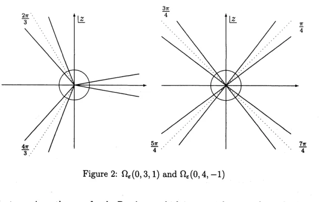
there exists a positive constant$\epsilon$ such that

(i) the Cauchy data $\varphi$ can be continued analytically in a domain

(3.10) $\Omega_{\epsilon}(d;q, \alpha):=\overline{\bigcup_{m=0}^{q1}}S(\frac{d+\arg\alpha+2\pi m}{q},$$\epsilon$,$\infty)$ ,

(ii) $\varphi$ has

a

growth condition

of

exponential order at most $q/(q-1)$, that is, there

eist positive constants $C$ and

7such

that the followinggrowth estimate holds.

(3.11) $|\varphi(z)|\leq C\exp(\gamma|z|^{q/(q-1)})$ , $z\in\Omega_{\epsilon}(d;q, \alpha)$

.

Figure 2: $\Omega_{\epsilon}(0,3,1)$ and 0,$(0, 4,$ $-1)$

Next, we giveatheorem for the Borel sum whichis aspecial

case

inthe author’s paper [Ich].

Theorem 3.3 (Ichinobe) Under the above conditions (i) and (ii) in Theorem 3.2, the

Borel sum $u_{B}^{d}(\tau, z)$ is given by the analytic continuation

of

the following

function

(3.12) $u_{B}^{d}( \tau, z)=\int_{0}^{\infty((d+\arg\alpha)/q)}\Phi_{q}(z, \zeta)k_{q}(\tau, \zeta;\alpha)d\zeta$, where $(\tau, z)\in 5(\mathrm{d}, \beta, \rho)\cross B_{f}$ with _{$\beta<(q-1)\pi$},

(3.13) $\Phi_{q}(z, \zeta)=\sum_{m=0}^{q-1}\varphi(z+\omega_{q}^{m}\zeta)$, $\omega_{q}=\exp(2\pi i/q)$,

and the kernel

_function

$k_{q}(\tau, \zeta;\alpha)$ is given by

(3.14) $k_{q}( \tau, \zeta;\alpha)=\frac{C_{q}}{\zeta}G_{0,q-1}^{q-1,0}(Z_{\alpha}|1/q,$ $2/q$,$\ldots$, $(q-1)/q)$ , with $Z_{\alpha}= \frac{1}{q^{q}\alpha}.\frac{\zeta^{q}}{\tau}$, $C_{q}= \frac{1}{\Pi_{j=1}^{q-1}\Gamma(j/q)}$.

In special

cases

the kernel functions

are

given

more

explicitly (cf.[LMS], [Ich])

Proposition 3.4 (i) When $(q, \alpha)=(2,1)$, that is, the case

of

the heat equation, the

kernel

_function

is given by

(3.15) $k_{2}( \tau, \zeta;1)=\frac{1}{\sqrt{4\pi\tau}}e^{-\zeta^{2}/4\tau}$

.

(ii) When $(q, \alpha)=(3,1)$, that is, the

case

of

the Airy equation, the kernel

function

is

given by

(3.16) $k_{3}( \tau, \zeta;1)=\frac{1}{(3\tau)^{1/3}}Ai(\frac{\zeta}{(3\tau)^{1/3}})$.

(iii) When $(q, \alpha)=(4, -1)$, that is, the case

of

the Beam equation, the kernel

function

is given by

(3.17) $k_{4}( \tau, \zeta;-1)=\frac{1}{(4\tau)^{1/4}}\frac{1}{2\pi i}\int_{\gamma_{2}}\exp[(\frac{\zeta}{(4\tau)^{1/4}})s-\frac{s^{4}}{4}]ds$,

where the path $\gamma_{2}$ is any

curve

which begins at infinity in the sector $7\pi/8<\arg s<$

$9\pi/8$ and ends at infinity in thesector$3\pi/8<\arg s<5\pi/8$ (see Figure 3at Section

4.2).

The statement (i) was given by [LMS] and the statement (ii)

was

given by [Ich]. The

statement (iii) is

anew

expression which will be proved in Section 5.

4Main result

As we have shown the Classical solution and the Borel

sum are

different notion and the

integral representations of solutions are also completely different, but we shall show a

relationship between these solutions as follows.

Claim The Classicalsolutions $u_{c}(t, x)$ are obtained by deforming the paths

of

integrations

for

the Borel sum $u_{B}^{0}(\tau, z)$ under some additional conditions

for

the Cauchy data, where

will be specified in each equation in the below.

4.1

Case of the

Airy

Equation

In Airy’s case, we recall the conditions for the Borel summability in 0direction for the

Cauchy data $\varphi(z)$ which is holomorphic in aneighbourhood ofthe origin.

The Cauchy data $\varphi(z)$ can be continued analytically in $\Omega_{\epsilon}(0;3,1)$ (see Figure 2) with

agrowth condition of exponential order at most 3/2 there

We recall the integral repesentation of the Borel sum $u_{B}^{0}(\tau, z)$

(4.1) $u_{B}^{0}(\tau, z)$ $=$ $\frac{1}{(3\tau)^{1/3}}\{\int_{0}^{+\infty}\varphi(z+\zeta)Ai(X)d\zeta$ $+ \int_{0}^{\infty(2\pi/3)}\varphi(z+()Ai(X\omega_{3}^{-1})\omega_{3}^{-1}d\zeta$

$+ \int_{0}^{\infty(4\pi/3)}\varphi(z+\zeta)Ai(X\omega_{3}^{-2})\omega_{3}^{-2}d\zeta\}$ , $X= \frac{\zeta}{(3\tau)^{1/3}}$,

where $(\tau, z)\in S(0,2\pi, \rho)\cross B_{r}$.

Now we

assume

the following additional conditions for the Cauchy data:

(1) $\varphi$ can be continued analytically in asector $S(\pi, 2\pi/3, \infty)$ with the

same

growth

condition

as

in the Borel summability.

(2) There exists apositive constant $\delta$ such that in the region _{$S(\pi, \delta, \infty)$},

$\varphi$ has

a

decreasing condition of polynomial order, exactly, there exist positive constants $C$

and Asuch that

$|\varphi(z)|\leq C|z|^{-3/4-\lambda}$, $z\in S(\pi, \delta, \infty)$

.

Under these assumptions, we can deform the paths of integrations as follows. First,

we restrict $\tau>0$ in the Borel

sum

$u_{B}^{0}(\tau, z)$

.

Then in the second and the third integrations

of the expression (4.1) the paths ofintegrations can be deformed into the integrations on

the negative axis, because the Airy function has the following asymptotic expansion (cf. [Erd, p. 96]$)$

.

(4.2) $Ai(z)= \frac{1}{2\sqrt{\pi}}z^{-1/4}\exp(-\frac{2}{3}z^{3/2})[1+O(z^{-3/2})]$ , $|\arg z|<\pi$, $zarrow\infty$

.

Therefore we have

(4.3) $u_{B}^{0}(\tau, z)$ $=$ $\frac{1}{(3\tau)^{1/3}}[\int_{0}^{+\infty}\varphi(z+\zeta)Ai(X)d\zeta$

$+ \int_{0}^{-\infty}\varphi(z+\zeta)\{Ai(X\omega_{3}^{-1})\omega_{3}^{-1}+Ai(X\omega_{3}^{-2})\omega_{3}^{-2}\}d\zeta]$ ,

where $\tau>0$ and $z\in \mathbb{R}$

.

Finally, by using the following functional equality of Airy

functions

(4.4) $w_{m}(z)+\omega_{3}w_{m+1}(z)+\omega_{3}^{2}w_{m+2}(z)=0$, $w_{m}(z)=Ai(\omega_{3}^{m}z)$,

(cf. [Erd, p.96]),

we

have

(4.3) $Ai(X\omega_{3}^{-1})\omega_{3}^{-1}+Ai(X\omega_{3}^{-2})\omega_{3}^{-2}=-Ai(X)$.

Therefore for $\tau>0$ and $z\in \mathbb{R}$ we obtain

(4.6) $u_{B}^{0}( \tau, z)=\frac{1}{(3\tau)^{1/3}}\int_{-\infty}^{+\infty}\varphi(z+\zeta)Ai(X)d\zeta$, $X= \frac{\zeta}{(3\tau)^{1/3}}$

.

4.2

Case

of the Beam

Equation

Before

we

give the integral representation of the Borel

sum

of the Beam equation $(\mathrm{B})_{\mathbb{C}}$,

we

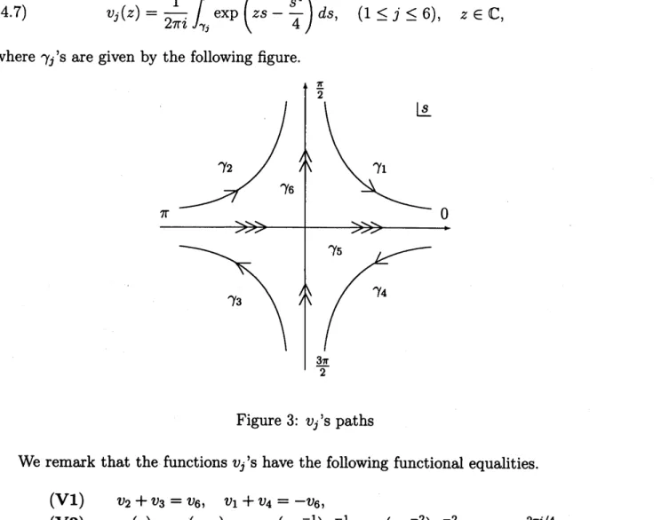
introduce the following functions.

(4.7) $v_{j}(z)= \frac{1}{2\pi i}\int_{\gamma_{j}}\exp(zs-\frac{s^{4}}{4})ds$, $(1\leq j\leq 6)$, $z\in \mathbb{C}$,

where $\gamma_{j}’ \mathrm{s}$ are given by the following figure.

Figure 3: $v_{j}’ \mathrm{s}$ paths

We remark that the functions $v_{j}’ \mathrm{s}$ have the following functional equalities.

(VI) $v_{2}+v_{3}=v_{6}$, $v_{1}+v_{4}=-v_{6}$,

(V2) $v_{2}(z)=v_{1}(z\omega_{4})\omega_{4}=v_{3}(z\omega_{4}^{-1})\omega_{4}^{-1}=v_{4}(z\omega_{4}^{-2})\omega_{4}^{-2}$, $\omega_{4}=e^{2\pi}:/4$

.

Moreover, there are the following relations between the kernel functions and the function

$v_{j}’ \mathrm{s}$, that is, the kernel function Be(z) of Classical solution (2.3) is _{$v_{6}(z)$}

(4.8) Be(z) $=v_{6}(z)$,

and the kernel function (3.17) of the Borel

sum

is given by $v_{2}$

(4.9) $k_{4}( \tau, \zeta;-1)=\frac{C_{4}}{\zeta}G_{0,3}^{3,0}(-\frac{\zeta^{4}}{4^{4}\tau}|1/4,2/4,3/4)=\frac{1}{(4\tau)^{1/4}}v_{2}(\frac{\zeta}{(4\tau)^{1/4}})$

.

From (4.8), the Classical solution is rewritten by

(4.10) $u_{c}^{B}(t, x)= \frac{1}{(4t)^{1/4}}\int_{-\infty}^{+\infty}\varphi(x+y)v_{6}(\frac{y}{(4t)^{1/4}})dy$,

where ${\rm Re} t>0$ and $x\in \mathbb{R}$.

Next, from (4.9) and Theorem 3.3, the Borel sum $u_{B}^{0}(\tau, z)$ of $(\mathrm{B})_{\mathbb{C}}$ is given by

(4.11) $u_{B}^{0}(\tau, z)$ $=$ $\frac{1}{(4\tau)^{1/4}}\{\int_{0}^{\infty(\pi/4)}\varphi(z+\zeta)v_{2}(X)d\zeta$

$+ \int_{0}^{\infty(3\pi/4)}\varphi(z+\zeta)v_{2}(X\omega_{4}^{-1})\omega_{4}^{-1}d\zeta+\int_{0}^{\infty(5\pi/4)}\varphi(z+\zeta)v_{2}(X\omega_{4}^{-2})\omega_{4}^{-2}d\zeta$

$+ \int_{0}^{\infty(7\pi/4)}\varphi(z+\zeta)v_{2}(X\omega_{4}^{-3})\omega_{4}^{-3}d\zeta\}$ , $X= \frac{\zeta}{(4\tau)^{1/4}}$,

where $(\tau, z)\in S(0,3\pi, \infty)\cross B_{f}$

.

By using the functional equalities (V2), the Borel sum $u_{B}^{0}(\tau, z)$ is rewritten in the

following form.

(4.12) $u_{B}^{0}(\tau, z)$

$=$ $\frac{1}{(4\tau)^{1/4}}\{$$\int_{0}^{\infty(\pi/4)}\varphi(z+\zeta)v_{2}(X)d\zeta+\int_{0}^{\infty(3\pi/4)}\varphi(z+\zeta)v_{1}(X)d\zeta$

$+ \int_{0}^{\infty(5\pi/4)}\varphi(z+\zeta)v_{4}(X)d\zeta+\int_{0}^{\infty(7\pi/4)}\varphi(z+\zeta)v_{3}(X)d\zeta\}$ .

We recall the conditions for the Borelsummability in 0direction for the Cauchy data.

The Cauchy data $\varphi(x)$ can be continued analytically in $\Omega_{\epsilon}(0;4, -1)$ (see Figure 2)

with agrowth condition ofexponential order at most 4/3 there.

We

assume

the following additional conditions for the Cauchy data:

$\bullet$ $\varphi$ can be continued analytically in asector $S(0, \pi/2, \infty)\cup S(\pi, \pi/2, \infty)$, and has

the

same

growth condition as in the Borel summability.

Then byrestricting${\rm Re}\tau>0$, we candeform thepathsofintegrations inthe Borelsum

as follows. The paths ofintegrations of the arguments $\pi/4$ and $7\pi/4$ can be changed into

the integrations

on

the positive real axis, and the paths of integrations of the arguments

$3\pi/4$ and $5\pi/4$ can be changed into the integrations on the negative real axis. In fact,

it follows from the expression (4.9) and the fact that the $G$-function has the following

asymptotic expansion (cf. [Luk, p. 179]).

(4.13) $G_{0,3}^{3,0}(z|1/4,$

$2/4$,

$3/4)$ $=$ $\frac{2\pi}{\sqrt{3}}z^{1/6}\exp(-3z^{1/3})[1+O(z^{-1/3})]$ ,

$zarrow\infty$, $|\arg z|\leq 4\pi-\delta$, $\delta>0$

.

Therefore we have

(4.14) $u_{B}^{0}(\tau, z)$ $=$ $\frac{1}{(4\tau)^{1/4}}[\int_{0}^{+\infty}\varphi(z+\zeta)\{v_{2}(X)+v_{3}(X)\}d\zeta$

$+ \int_{0}^{-\infty}\varphi(z+\zeta)\{v_{1}(X)+v_{4}(X)\}d\zeta]$ ,

where ${\rm Re}\tau>0$ and $z\in \mathbb{R}$. Finally, by using the functional equalities (VI), we obtain (4.15) $u_{B}^{0}( \tau, z)=\frac{1}{(4\tau)^{1/4}}\int_{-\infty}^{+\infty}\varphi(z+\zeta)v_{6}(X)d\zeta$, $X= \frac{\zeta}{(4\tau)^{1/4}}$.

Therefore $u_{c}^{B}(t, x)=u_{B}^{0}(t, x)$ by restricting $t>0$ and $x\in \mathbb{R}$ in the above formula.

5Sketch of Proof of Proposition 3.4,

(iii)

We shall prove the statement (iii) of Proposition 3.4 which

means

(5.1) $\frac{C_{4}}{\zeta}G_{0,3}^{3,0}(Z_{-1}|1/4,2/4,3/4)=\frac{1}{(4\tau)^{1/4}}\frac{1}{2\pi i}\int_{\gamma 2}\exp[(\frac{\zeta}{(4\tau)^{1/4}})s-\frac{s^{4}}{4}]ds$,

where $Z_{-1}=\zeta^{4}/(4^{4}e^{\pi i}\tau)$ (since $ce=-1=e^{\pi i}$) and _{$C_{4}= \prod_{j=1}^{3}\Gamma(j/4)$}

.

We recall the following formula for the $G$-function(cf. [Luk, p. 150])

(5.2) $z^{\sigma}G_{p,q}^{m,n}(z|\alpha\gamma)=G_{\mathrm{p},q}^{m,n}(z|\alpha+\sigma\gamma+\sigma)$ ,

where $\alpha+\sigma=$ $(\alpha_{1}+\sigma, \alpha_{2}+\sigma, \ldots, \alpha_{p}+\sigma)$. Then we have

$\frac{C_{4}}{\zeta}G_{0,3}^{3,0}(Z_{-1}|1/4,2/4,3/4)=\frac{1}{(4\tau)^{1/4}}\frac{C_{4}e^{-\pi i/4}}{4^{3/4}}Z_{-1}^{-1/4}G_{0,3}^{3,0}(Z_{-1}|1/4,2/4,3/4)$

$= \frac{1}{(4\tau)^{1/4}}\frac{C_{4}e^{-\pi i/4}}{4^{3/4}}G_{0,3}^{3,0}(Z_{-1}|0,1/4,2/4)$ .

Therefore it is enough to prove the following equality

(5.3) $\frac{C_{4}e^{-\pi\dot{l}/4}}{4^{3/4}}G_{0,3}^{3,0}(Z_{-1}|0,1/4,2/4)=\frac{1}{2\pi i}\int_{\gamma 2}\exp[(\frac{\zeta}{(4\tau)^{1/4}})s-\frac{s^{4}}{4}]ds$.

In order to do so, we shall show that the power series expansions of both sides are the

same ones. Precisely, we give the power series expansion at $Z_{-1}=0$ of the left hanc

side and at $\zeta/(4\tau)^{1/4}=X=0$ of the right hand side, respectively. We note the relation

between $Z_{-1}$ and $X$,

$Z_{-1}= \frac{1}{4^{3}e^{\pi i}}X^{4}$

(or

$X=4^{3/4}e^{\pi i/4}Z_{-1}^{1/4}$

).

First, from the integral representation of the $G$-function

on

the left hand side of (5.3)

we have the following expansion by calculating the residues ofthe left side ofthe path of integration $I=\{{\rm Re} s=\kappa;\kappa>0\}$.

(5.4) $G_{0,3}^{3,0}(Z_{-1}|0,$ $1/4$, $2/4)= \frac{1}{2\pi i}\int_{I}\Gamma(s)\Gamma(1/4+s)\Gamma(2/4+s)Z_{-1}^{-s}ds$ $=$ $\sum_{\ell=1j}^{3}\prod_{=1,j\neq\ell}^{3}\Gamma(\frac{j-\ell}{4})Z_{-11}^{(\ell-1)/4}F_{3}((1+\ell)/4,$ _{$(2+\ell)/41$} , $(3+\ell)/4$ ; $(-1)^{3}Z_{-1})$

.

Next, onthe right hand side of(5.3), by expanding$e^{Xs}$ in the integrand into itspower

series and by termwise integrating, we have

$\frac{1}{2\pi i}\int_{\gamma 2}\exp[Xs-\frac{s^{4}}{4}]ds=\frac{1}{2\pi i}\sum_{n=0}^{\infty}\frac{X^{n}}{n!}\int_{\gamma 2}s^{n}\exp(-\frac{s^{4}}{4})ds$

.

We choose the path of integration $\gamma_{2}$

as

the summation of two rays with the arguments

$\pi/2$ and $\pi$

.

Then these integrals

can

be expressed in terms of the gamma functions.

$\frac{1}{2\pi i}\sum_{n=0}^{\infty}\frac{X^{n}}{n!}\int_{\gamma 2}s^{n}\exp(-\frac{s^{4}}{4})ds$

$=$ $\frac{1}{2\pi i}\sum_{n=0}^{\infty}\frac{X^{n}}{n!}\{\int_{0}^{\infty(\pi/2)}-\int_{0}^{\infty(\pi)}\}_{1}s^{n}\exp(-\frac{s^{4}}{4})ds$

$=$ $\frac{1}{2\pi i}\sum_{n=0}^{\infty}\frac{X^{n}}{n!}\{e^{\pi i(n+1)/2}-e^{\pi i(n+1)/4}\}4^{(n-3)/4}\Gamma(1+\frac{n-3}{4})$

$=$ -$\sum_{n=0}^{\infty}\frac{X^{n}}{n!}\frac{4^{(n-3)/4}e^{3\pi i(n+1)/4}}{\Gamma(1-(n+1)/4)}$

.

The third equality is obtained from the following relations

$e^{\pi i(n+1)/2}-e^{\pi i(n+1)/4}$ _$=$ $-e^{3:(n+1)/4}(\pi e^{\pi i(n+1)/4}-e^{-\pi i(n+1)/4})$

$=$ $-e^{3\pi i(n+1)/4}2i \mathrm{s}.\mathrm{n}(\frac{n+1}{4}\pi)$ $2\pi ie^{3\pi i(n+1)/4}$ $=$

$-_{\overline{\Gamma((n+1)/4)\Gamma(1-(n+1)/4)}}$.

When $n=4k+3$ in the abovesummation,

we

notice $1/\Gamma(1-(n-1)/4)=1/\Gamma(-k)=0$.

Therefore by calculating carefully, we have

(5.5) -$\sum_{n=0}^{\infty}\frac{X^{n}}{n!}\frac{4^{(n-3)/4}e^{3\pi i(n+1)/4}}{\Gamma(1-(n+1)/4)}$

$=$ -$\sum_{\ell=0}^{2}\sum_{k=0}^{\infty}\frac{X^{4k+\ell}}{(4k+\ell)!}\frac{4^{k+(\ell-3)/4}e^{3\pi i(\ell+1)/4}(-1)^{k}}{\Gamma(1-k-(\ell+1)/4)}$

$=$ -$\sum_{\ell=0}^{2}\frac{e^{3\pi 1(\ell+1)/4}4^{(\ell-3)/4}X^{\ell}}{\Gamma((3-\ell)/4)\ell!}1F3((\ell+2)/4,$ _{$(\ell+3)/41$}

, $(\ell+4)/4$ ; $\frac{X^{4}}{4^{3}})$ $=$ - $\sum_{\ell=1}^{3}\frac{e^{3\pi i\ell/4}4^{(\ell-4)/4}X^{\ell-1}}{\Gamma((4-\ell)/4)(\ell-1)!}1F3$

(

$(\ell+1)/4$, $(\ell+2)/41$ , $(\ell+3)/4$ ; $\frac{X^{4}}{43}$

).

The second equality is obtained from the relations

$(4k+\ell)!$ $=$ $4^{4k}( \frac{\ell+1}{4})_{k}(\frac{\ell+2}{4})_{k}(\frac{\ell+3}{4})_{k}(\frac{\ell+4}{4})_{k}\ell!$,

$\Gamma(1-\frac{\ell+1}{4}-k)$ $=$ $\Gamma(\frac{3-\ell}{4}-k)=\Gamma(\frac{3-\ell}{4})/(-1)^{k}(\frac{\ell+1}{4})_{k}$,

and by employing the representation (3.8) of the generalized hypergeometric series.

At the end the proof is comlete by examing the following relations.

$(-1)^{3}Z_{-1}= \frac{\zeta^{4}}{4^{4}t}=\frac{X^{4}}{4^{3}}(X=\frac{\zeta}{(4\tau)^{1/4}})$ , $Z_{-1}^{1/4}= \frac{1}{4^{3/4}e^{\pi i/4}}X$,

and

$C_{4} \cross\prod_{j=1,j\neq\ell}^{3}\Gamma(\frac{j-\ell}{4})$ $= \prod_{j=1}^{3}\Gamma(\frac{j}{4})\cross\prod_{j=1,j\neq\ell}^{3}\Gamma(\frac{j-\ell}{4})$

$=$ $\frac{(-1)^{\ell-1}4^{\ell-1}}{(\ell-1)!}\frac{1}{\Gamma(1-\ell/4)}=\mathrm{i}_{\frac{1}{\Gamma(1-\ell/4)}}e^{(\ell-1)\pi}4^{\ell-1}(\ell-1)!$

which is obtained from the multiplication formula for the gamma function (cf. [Luk, $\mathrm{p}$,

11])

(5.6) $\Gamma(mz)=(2\pi)^{-(m-1)/2}m^{mz-1/2}\prod_{j=0}^{m-1}\Gamma(z+\frac{j}{m})$ ,

where $z+j/m\not\in \mathbb{Z}_{\leq 0}:=\{0,$-1, -2,

. . ,}

(j $=0,$ 1,\ldots ,m-1).

6Generalization of

our

Claim

In this section, we shall give ageneralization ofour claim $(q=3,4)$ as atheorem without

proof which will be given in aforthcoming paper.

We consider the following Cauchy problems

$(\mathrm{C}\mathrm{P})_{\mathrm{R}}$ $\partial_{t}u(t, x)=\alpha\partial_{x}^{q}u(t, x)$, $5(0, x)=\varphi(x)$, $t>0$, $x\in \mathbb{R}$,

$(\mathrm{C}\mathrm{P})_{\mathbb{C}}$ $\partial_{\tau}u(\tau, z)=\alpha\partial_{z}^{q}u(\tau, z)$, $u(0, z)=\varphi(z)$, $\tau$, $z\in \mathbb{C}$,

where $q\geq 4$, $\alpha=1$ if$q\not\in 4\mathbb{Z}$ and $ce=-1$ if $q\in 4\mathbb{Z}$.

Under the above assumptions the Cauchy problem $(\mathrm{C}\mathrm{P})\mathrm{r}$ is uniquely solvable in $S$

and the Classical solution $u_{c}(t, x)$ is given by

(6.1) $uc(t, x)= \int_{-\infty}^{+\infty}\varphi(x+\mathrm{u}\mathrm{c}(\mathrm{t}, y)dy,$ $t>0$, $x\in \mathbb{R}$

.

Here the kernel function $E(t, y)$ is given by

(6.2) $E(t, y)=\{$

$\frac{1}{(qt)^{1/q}}\frac{1}{2\pi i}\int_{\mathrm{y}},\exp(\frac{y}{(qt)^{1/q}}s-\frac{s^{q}}{q})ds$, if $q\neq 4n+2$,

$\frac{1}{(qt)^{1/q}}\frac{1}{2\pi i}\int_{-i\infty}^{+i\infty}\exp(\frac{y}{(qt)^{1/q}}s+\frac{s^{q}}{q})ds$, if $q=4n+2$ ,

where $\gamma$ is given as follows:

(I) When

_$q=4n-1$

, the path $\gamma$ is any

curve

which begins at

oo

in the sector

$3\pi/2-\pi/q<\arg s<3\pi/2$ _{and ends at} $\infty$ in the sector $\pi/2<\arg s<\pi+\pi/q$. (II) When $q=4n$, the path $\gamma$ runs $\mathrm{f}\mathrm{r}\mathrm{o}\mathrm{m}-i\infty \mathrm{t}\mathrm{o}+i\infty$.

( $(\mathrm{I})$ When $q=4n+1$, the path

$\gamma$ is any curve which begins at oo in the sector

$3\pi/2<\arg s<3\pi/2+\pi/q$ and ends at $\infty$ in the sector $\pi/2-\pi/q<\arg s<\pi/2$

.

Now,

our

theorem for the relationship between the Classical solution $u_{c}(t, x)$ which is

given by (6.1) and the Borel sum $u_{B}^{0}(\tau, z)$ which is given by (3.12) is stated as follows.

Theorem 6.1 Under the additional conditions

_for

the Cauchy data which

are

stated

be-low, the expressions (6.1)

_of

the Classical solutions $u_{c}(t, x)$ are obtained by deforming the

paths

_of

integrations (3.12)

_for

the Borel

sum

$u_{B}^{0}(\tau, z)$

.

(I) (Generalization

_of

Airy equation) When

$q=4n-1$

, the Cauchy data $\varphi$

can

be

continued analytically in a sector $S(0, \pi-3\pi/q, \infty)\cup S(\pi, \pi-\pi/q, \infty)$ with the

same growth condition as in the Borel summability in Theorem 3.3 and there exists

a positive constant $\delta$ such that in the region $S(\pi, \delta, \infty)$, $\varphi$ has a decreasing condition

of

polynomial order, exactly, there exist positive constants $C$ and Asuch that

(6.3) $|\varphi(z)|\leq C|z|^{-3/2(q-1)-\lambda}$.

(II) (Generalization

_of

the heat equation) When $q=2n$, the Cauchy data $\varphi$ can be

continued analytically in a sector $S(0, \pi-2\pi/q, \infty)\cup S(\pi, \pi-2\pi/q, \infty)$ $with$ the

same

growth condition as in the Borel summability in Theorem 3.3.

(II) When $q=4n+1$, the Cauchy data $\varphi$ can be continued analytically in a sector

$5(0, \pi-\pi/q, \infty)\cup S(\pi, \pi-3\pi/q, \infty)$ with the

same

growth condition

as

in the Borel summability in Theorem 3.3 and there exists a positive constant $\delta$ such that in the

region$S(0, \delta, \infty)$, $\varphi$ has the

same

decreasing condition (6.3) as in the

case

$q=4n-1$

.

References

[Bal] W. Balser, Prom Divergent Power Series to Analytic Functions, Springer Lecture

Notes, No. 1582, 1994.

[Erd] A. Erdelyi, Asymptotic Expansion, Dover

1956.

[Ich] K. Ichinobe, The Borel Sum

_of

Divergent Barnes Hypergeometric Series and its

Application to a Partial

_Differential

Equation, Publ. ${\rm Res}$. lust. Math. Sci., 37 (2001),

No. 1, _91-117.

[LMS] D. Luts, M. Miyake and R. Sch\"aflce, On the Borel summability

_of

divergent solu-tions

_of

the heat equation, Nagoya Math. J., 154 (1999), 1-29.

[Luk] Y. L. Luke, The Special Puctions and Their Approximations, Vol IAcademic Press,

1969.

[Miy] M. Miyake, Borel summability of divergent solutions of the Cauchy problem to

non-Kowalevskian equations, Partial differential equations and their applications

(Wuhan,1999), 225-239, World Sci. Publishing River Edge,NJ,1999.

[MS] A. M. Mathai and R. K. Saxena, Generalized Hypergeometric Functions with

Applications in Statistics and P hysical Sciences, Springer Lecture Notes. No. 348, 1973