Stability of Delaunay surfaces as steady states for a geometric evolution equation (Singularity theory of differential maps and its applications)

全文

(1)57. 数理解析研究所講究録第2049巻 2017年 57-70. of. Stability for. Delaunay surfaces. as. steady. states. geometric evolution equation. a. Yoshihito Kohsaka Graduate School of Maritime. Sciences,. Let $\Gamma$_{t} \subset \mathbb{R}^{3} be. a. evolving surface with respect. to time t. V=-$\Delta$_{$\Gamma$_{t}}H one. mean. on. .. The surface diffusion. equation. (1). $\Gamma$_{t}. of the. geometric evolution laws, where V is the normal velocity of $\Gamma$_{t}, H is the mean $\Gamma$_{t} and $\Delta$_{$\Gamma$_{t} is the Laplace‐Beltrami operator on $\Gamma$_{t} In our sign convention, the curvature H for spheres with outer unit normal is negative.. curvature of. The. mean. ,. .. curvature flow. V=H is. University. Introduction. 1. is. Kobe. well‐known. law and. on. (2). $\Gamma$_{t}. the L^{2} ‐gradient flow for the. functional. geometric represented implies a variational structure that the area of the surface $\Gamma$_{t} decreases with respect to time t On the other hand, the surface diffusion equation (1) is the H^{-1} ‐gradient flow for the area functional of $\Gamma$_{t} so that this geometric evolution equation has a variational structure that the area of the surface $\Gamma$_{t} decreases with respect to time t whereas the volume of the region enclosed by the surface $\Gamma$_{t} is preserved. In this paper, we consider the following problem. For $\phi$\pm : \mathbb{R}_{+}\rightar ow \mathbb{R} set a. of $\Gamma$_{t}. .. as. area. This. .. ,. ,. $\Pi$_{\pm}=\{($\phi$_{\pm}(| $\eta$|), $\eta$)^{T}| $\eta$\in \mathbb{R}^{2}\}, $\Omega$=\{(x, $\eta$)^{T}|$\phi$_{-}(| $\eta$|)\leq x\leq$\phi$_{+}(| $\eta$|), $\eta$\in \mathbb{R}^{2}\}, \partial $\Omega$=\mathrm{I}\mathrm{I}_{-\cup$\Pi$_{+} . Note that. $\Pi$_{\pm} are the axisymmetric surfaces. Let $\Gamma$_{t} is governed by. Here, N_{$\Gamma$_{t} and N_{$\Pi$_{\pm}}. are. outer unit co‐normals to. us assume. that. \left{bginary}{l V=-$\Deta_{Gm$\athrm{}H\athrm{o} n$\Gam _{t},\ (N$Gam _{i},N$\Gam 1p})_{\mathrR}^{3=\cos$thea_{\pm} thr{o\ma n}$Gma_{t}\cp$Pi m},\ (nabl_{$\Gmat}H,\mhr{v}_pm)\athr{R}^3=0\mathr{o} mn$\Ga _{t}cp$\Pi m}, $\Gam_{t}|=0$\Gam _{0}. \endary}ight.. the outer unit normals to $\Gamma$_{t} and $\Pi$_{\pm} ,. \partial$\Gamma$_{t}. on. $\Gamma$_{t}\cap \mathrm{I}\mathrm{I}_{\pm}.. $\Gamma$_{t} \subset $\Omega$ and the motion of. respectively,. (3) and $\nu$\pm. are. the.

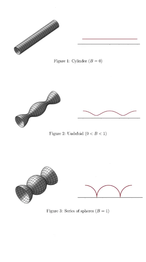
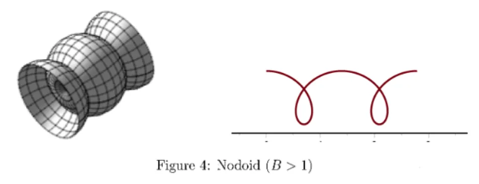
(2) 58. Let $\Gamma$_{*} be the. steady. states for. (3). and H. be the. mean. curvature of. $\Gamma$_{*} Then $\Gamma$_{*} satisfies .. \left\{begin{ar y}{l $\Delta$_{\Gam a$_{*}H_{*}=0\mathrm{o}\mathrm{n}$\Gam a$_{*},\ (\nabl_{$\Gam a$_{*}H_{*},$\nu$_{\pm})\mathrm{l}\mathrm{R}^\mathrm{s}=0 \mathrm{o}\mathrm{n}$\Gam a$_{*}\cap$\Pi$_{\pm}. \end{ar y}\right. Multiplying H_{*} by the we. both side of the. equation $\Delta$_{$\Gamma$_{*}}H_{*}=0 and applying the Greens formula,. obtain. \Vert\nabla_{$\Gamma$_{*} H_{*}\Vert_{L^{2}($\Gamma$_{*})}^{2}=0. steady states of (3) are the constant mean curvature surfaces (CMC surfaces). In this paper, we only consider the axisymmetric CMC surfaces, which is so called the Dclaunay surfaces, as the steady states $\Gamma$_{*} For an axisymmctric perturbation from $\Gamma$_{*}, we derive the eigenvalue problem corresponding to the linearized problem for (3) and obtain the criteria of the stability of $\Gamma$_{*}. As regards the results on the stability of the Delaunay surfaces as the variational problem for the capillary energy, we refer to Athanassenas [2], Fel and Rubinstein [6, 14], and Vogel [15, 16, 17, 18, 19]. Concerning the results on the stability as steady states for the surface diffusion equation, we refer to Abels, Garcke, and Müller [1], Depner [5], and LeCrone and Thus. we see. that the. .. [12].. Simonctt. The. 2. Let $\Gamma$_{*} be. a. eigenvalue problem axisymmctric steady. states of. (3). and set. $\Gamma$_{*}=\{ (x_{*}(s), y_{*}(s)\cos $\zeta$, y_{*}(s)\sin $\zeta$)^{T}|s\in[0, d] , $\zeta$\in[0, 2 $\pi$ where. is the. s. theorem, constant. we. mean. Theorem 2.1 a. generating. arc‐length parameter. introduce the. of. a. generating. curve. (x_{*}(s), y_{*}(s))^{T}. .. In the. representation formula of the Delaunay surfaces with. following. a non‐zero. curvature.. ([9, 13]) Let H_{*} be a constant satisfying H_{*}\neq 0 (assuming H_{*}<0 ). Then (x_{*}(s), y_{*}(s))^{T} of the Delaunay surface with a constant mean curvature. curve. H_{*} is given by. where. B\geq 0 and $\tau$\in \mathbb{R}. The a. \left{\begin{ar y}{l x_{*}(s)=\int_{0}^s\frac{1-B\sin(2H_{*}($\sigma$- \tau$)}{\sqrt{1+B^{2}-B\sin(2H_{*}($\sigma$- \tau$)}d$\sigma$,\ y_{*}(s)=-\frac{1}2H_{*}\sqrt{1+B^{2}-B\sin(2H_{*}(s-$\tau$)}, \end{ar y}\right. are. (4). constants.. Delaunay surface is a cylinder for B=0 (Fig. 1), an unduloid for 0<B<1 (Fig. 2), spheres for B=1 (Fig. 3), and a nodoid for B>1 (Fig. 4).. series of.

(3) 59. Figure. Figure. Figure. 1:. Cylinder (B=0). 2: Unduloid. 3: Series of. (0< B < 1). spheres (B=1).

(4) 60. Figure. Applying ing the. where. an. 4: Nodoid. (B> 1). axisymmetric perturbation v(s, t) for the Delaunay surfaces $\Gamma$_{*} and lineariz‐ problem for v(s, t) we have. nonlinear. ,. \left{bgin{ary}l v_{t}=-\frac{1}2$\Delta$_{\Gam $_{*}L[v]\mathr{f}\mathr{o}\mathr{}(s,t)\in[0,d]\times[0,T]\ partil_{s}v\pm($kap $_{\Pi$_{pm}\cs$thea$_{\pm}-$kap $_{\Gam $_{*}\cot$hea$_{\pm})v=0\mathr{f}\mathr{o}\mathr{}s=0,dt\in[0,T]\ partil_{s}L[v]=0\mathr{f}\mathr{o}\mathr{}s=0,dt\in[0,T] \end{ary}\ight.. L[v] =$\Delta$_{$\Gamma$_{*}}v+|A_{*}|^{2}v. (5). with. $\Delta$_{$\Gamma$_{*} =\displaystyle \frac{1}{y_{*} \{\partial_{s}(y_{*}\partial_{s})+\frac{1}{y_{*} \partial_{ $\zeta$}^{2}\}, |A_{*}|^{2}=(-x_{*}'y_{*}'+x_{*}'y_{*}')^{2}+ (\frac{x_{*}' {y_{*} )^{2} and. $\kap a$_{$\Pi$_{\pm} =\displaystyle\pm\frac{\d ot{$\phi$}_{\pm}(y_{*}) {\ 1+(\dot{$\phi$}_{\pm}(y_{*}) ^{2}\ ^{3/2} ,$\kap a$_{$\Gam a$_{*} =-x_{*}'y_{*}'+x_{*}'y_{*}'. Note that $\kappa$_{$\Pi$_{-} and $\kappa$_{$\Pi$_{-} at y. are. the curvature of. x. =y_{*}(d) respectively,. Taking. =. -$\phi$_{-}(y). at y. =. and $\kap a$_{$\Gamma$_{*} is the curvature of the generating account of the fact that v is independent of $\zeta$ , we have ,. y_{*}(0). and. curve. x. =. $\phi$_{+}(y). (x_{*}(s), y_{*}(s))^{T}.. $\Delta$_{$\Gam a$_{*} v=\displaystyle\frac{1}{y_{*} \{ partial_{s}(y_{*}\partial_{s}v)\}. For this linearized. problem. thc. corresponding eigenvalue problem. is. given by. \left{begin{ar y}{l -$\Delta$_{\Gam $_{*}L[w]=$\lambd$w\mathr{f}\mathr{o}\mathr{}s\in[0,d]\ partil_{s}w\pm($\kap $_{\Pi$_{pm}\cs$thea$_{\pm}-$\kap $_{\Gam $_{*}\cot$ hea$_{\pm})w=0\mathr{a}\mthr{}s=0,d\ partil_{s}L[w]=0\mathr{a}\mthr{}s=0,d. \end{ar y}\ight.. We say that the steady states $\Gamma$_{*} is only if all of eigenvalues of (6) are. linearly stable negative.. under. an. (6). axisymmetric perturbation if and.

(5) 61. Set. \displaystyle \mathcal{E}=\{w\in H^{1}($\Gamma$_{*})| \int_{0}^{d}wy_{*}ds=0\}, \mathcal{X}=\{w\in(H^{1}($\Gamma$_{*}))^{*}|\langle w, 1\}=0 (H^{1}($\Gamma$_{*}))^{*} is H^{1}($\Gamma$_{*}) Also, set. where. the. duality. space of. H^{1}($\Gamma$_{*}). and. \rangle. duality pairing (H^{1}($\Gamma$_{*}))^{*} and. is the. .. \mathcal{D}(\mathcal{A})=\{w\in H^{3}($\Gamma$_{*})|w. satisfies. \partial_{s}w\pm($\kappa$_{\mathrm{I}\mathrm{I}\pm}\csc$\theta$_{\pm}-$\kappa$_{$\Gamma$_{*} \cot$\theta$_{\pm})w=0 and. Taking. ,. s=0, d,. \displaystyle \int_{0}^{d}wy_{*}ds=0\}. and define the linear operator \mathcal{A}. \langle Aw. at. :. \mathcal{D}(\mathcal{A})\rightar ow \mathcal{X} by. $\psi$\displaystyle \rangle=\int_{0}^{d}\partial_{s}L[w]\partial_{s} $\psi$ y_{*}ds (w\in D(\mathcal{A}), $\psi$\in \mathcal{E}). .. symmetric bilincar form. thc. I[w_{1}, w_{2}]=\displaystyle \int_{0}^{d}\{\partial_{s}w_{1}\partial_{s}w_{2}-|A_{*}|^{2}w_{1}w_{2}\}y_{*}ds. +y_{*}($\kappa$_{$\Pi$_{+} \csc$\theta$_{+}-$\kappa$_{ $\Gamma$}. \cot$\theta$_{+})w_{1}w_{2}|_{s=d} +y_{*}($\kappa$_{$\Pi$_{-} \csc$\theta$_{-}-$\kappa$_{$\Gamma$_{*} \cot$\theta$_{-})w_{1}w_{2}|_{s=0},. and the H^{-1} ‐inner. product. (w_{1}, w_{2})_{-1}=\displaystyle \int_{0}^{d}2, where u_{wi} is. a. weak solution of. \left\{ begin{ar y}{l -$\Delta$_{ \Gam a$_{*}u_{wi}=w_{i}\mathrm{f}\mathrm{o}\mathrm{r}s\in(0,d),\ \parti l_{s}u_{w_{i}=0\mathrm{a}\mathrm{t}s=0,d \end{ar y}\right. for w_{i}\in \mathcal{X}. ,. we. obtain. (\mathcal{A}w, $\psi$)_{-1}=-I[w, $\psi$] ( $\psi$\in \mathcal{E}) For the linear operator \mathcal{A} and its. eigenvalues,. (P1). The operator A is. (P2). The spectrum of \mathcal{A} contains. self‐adjoint a. we. have the. .. following properties.. with respect to the H^{-1} ‐inner countable system of real. product.. eigenvalues..

(6) 62. (P3). \{$\lambda$_{n}\}_{n\in \mathrm{N}. Let. be. characterized. eigenvalues of A with $\lambda$_{1} \geq $\lambda$_{2} \geq $\lambda$_{3} \geq. Then. \ldots. .. \{$\lambda$_{n}\}_{n\in \mathrm{N}. are. by. $\lambda$_{1}=-\displaystyle \inf_{w\in \mathcal{E}\backslash \{0\} \frac{I[w,w]}{(w,w)_{-1} , \mathcal{W}\in$\Sigma$_{n-1}\inf_{w\in \mathcal{W}^{\perp}\backslash \{0\} \frac{I[w,w]}{(w,w)_{-1} . $\lambda$_{n}=- \displaystyle \sup. Here, $\Sigma$_{n} is the class of subspaces of \mathcal{E} with n‐dimension and \mathcal{W}^{\perp} subspace of \mathcal{W} with respect to the H^{-1} ‐inner product.. (P4). The. eigenvalues of \mathcal{A} depend continuously decreasing with respect to $\kap a$_{\mathrm{I}\mathrm{I}\pm}.. Concerning proofs,. 3. see. Criteria of. [5, 8]. for. (P1). and. (P2),. on. and. $\kappa \Pi$_{\pm}, $\kap a$_{$\Gamma$_{ $\rho$} ., d , and. [4, Chapter VI]. is the. $\theta$_{\pm} and ,. for. (P3). are. and. monotone. (P4).. Stability. If the maximal an. orthogonal. eigenvalue $\lambda$_{1} for (6) is negative, the steady states $\Gamma$_{*} are linearly axisymmetric perturbation. First, we show the following lcmma.. stable under. Lemma 3.1 Set. $\Lambda$\pm:=$\kappa$_{\mathrm{I}\mathrm{I}\pm}\csc$\theta$_{\pm}-$\kappa$_{$\Gamma$_{*} \cot$\theta$_{\pm}. Then there exists m>0 and $\delta$>0 such that. I[w, w]>0 (w\in \mathcal{E}\backslash \{0\}). ,. provided that $\Lambda$_{-}, $\Lambda$_{+}>m and d< $\delta$. proof, see [10]. implies that there exist m> 0 and \overline{ $\delta$}> 0 such that the maximal cigenvalue $\lambda$_{1} is non‐positive, provided that $\kap a$_{\mathrm{I}\mathrm{I}_{-} , $\kappa$_{$\Pi$_{+} > m and d < $\delta$ That is, all of eigenvalues are non‐positive. According to (P4), the eigenvalues depend continuously on the parameters and are monotone decreasing with respect to $\kap a$_{\mathrm{I}\mathrm{I}\pm} Thus we want to know the condition for the parameters that the zero is an eigenvalue for the eigenvalue problem (6). Now we consider thc zero‐eigenvalue problem. Regarding. a. Lcmma 3.1. .. .. $\Delta$_{$\Gamma$_{*}}L[w]=0 for s\in[0, d] \partial_{s}w\pm($\kappa$_{$\Pi$_{\pm}}\csc$\theta$_{\pm}-$\kappa$_{$\Gamma$_{*} \cot$\theta$_{\pm})w=0 \partial_{s}L[w]=0 at s=0, d. (7) (8) (9). ). at. s=0,. d. ,. .. Multiplying L[w] by. the both side of. (7). and. integrating. \Vert\partial_{s}L[w]\Vert_{L^{2}($\Gamma$_{*})}^{2}=0.. it. by parts. with. (9),. we. have.

(7) 63. Hence. L[w]. boundary. must be. constants,. (9). condition. if. we. so. that. we. can. obtain the solutions of. L[w]=0, L[w]= $\gamma$(\neq 0). Let w_{1}, w_{2} be fundamental solutions of L[v] =0 and w3 be a solution of (7) satisfying the boundary condition (9) is represented by. w(s)=c_{1}w_{1}(s)+c_{2}w_{2}(s)+c_{3}w_{3}(s) (i = 1,2,3). given by (11). is. a. arc. the. (10). .. solution of. where \mathrm{c}_{\mathrm{z}. (7) satisfying. solve. arbitrary. L[v]. = $\gamma$. .. Then. (11). ,. Deriving the condition of parameters satisfying the boundary condition (8) and. constants.. non‐trivial solution. a. that. w. \displaystyle \int_{0}^{d}vy_{*}ds=0, it. is. gives the condition of parameters that the zero is an cigenvalue if and only if the parameters satisfy. an. eigenvalue for (6).. That. \left|bgin{ary}l w_{1}'(0)-$\Lambd$_{-}w1(0)&w_{2}'(0)-$\Lambd$_{-}w2(0)&w_{3}'(0)-$\Lambd$_{-}w3(0)\ w_{1}'(d)+$\Lambd$_{+}w1(d)&w_{2}'(d)+$\Lambd$_{+}w2(d)&w_{3}'(d)+$\Lambd$_{+}w3(d)\ int_{0}^dw_{1}y*d_{9}&\int_{0}^dw_{2}y*ds&\int_{0}^duf}3y_{*d\mathcl{S} \end{ary}\ight|=0. is, the. ,. zero. (12). \mathrm{w}\mathrm{h}_{\mathrm{C}^{\backslash } \mathrm{r}\mathrm{c}$\Lambda$_{\pm}=$\kap a$_{ $\Gamma$ \mathrm{I}\pm}\csc$\theta$_{\pm}-$\kap a$_{$\Gamma$_{*} \cot$\theta$_{\pm} Setting .. w(s)=(w_{1}(s), w_{2}(s), w_{3}(s) ^{T}, (12). is. equivalent. I(d)=. (\displaystyle \int_{0}^{d}w_{1}y_{*}ds, \int_{0}^{d}w_{2}y_{*}ds, \int_{0}^{d}w_{3}y_{*}ds)^{T}. to. A^{w}$\kappa$_{$\Pi$_{-} $\kappa$_{$\Pi$_{+} +B_{-}^{w}$\kappa$_{$\Pi$_{-} +B_{+}^{w}$\kappa$_{$\Pi$_{+} +C^{w}=0. ,. where. A^{w}= - (w(0)\times w(d), I(d))_{\mathrm{R}^{3}},. B_{-}^{w}=\{-(w(0)\times w'(d), I(d))_{1\mathrm{R}^{3}}+(w(0)\times w(d), I(d))_{\mathrm{R}^{3}}$\kappa$_{$\Gamma$_{*}}(d)\cot$\theta$_{+}\}\sin$\theta$_{+}, B_{+}^{w}=\{ (w'(0) \times w(d), I(d))_{\mathrm{N}^{3}}+(w(0)\times w(d), I(d))_{\mathrm{R}^{3}}$\kappa$_{$\Gamma$_{*}}(0)\cot$\theta$_{-}\}\sin$\theta$_{-}, C^{w}=\{(w'(0)\times w'(d), I(d))_{\mathbb{R}^{3}} - (w(0)\times w(d), I(d))_{\mathrm{R}^{3} $\kappa$_{$\Gamma$_{*} (d)$\kappa$_{ $\Gamma$}.(0)\cot$\theta$_{+}\cot$\theta$_{-}\}\sin$\theta$_{+}\sin$\theta$_{-}. Then. we. (I). A^{w}\neq 0. If. obtain the and. following three representaitons of (13).. B^{\underline{w}}B_{+}^{w}-A^{w}C^{w}\neq 0,. (13). \Leftrightar ow. $\kap $_{\Pi$_{+}=-\displayte\frac{B^\underli {w} A^{w}+\frac{ B^{\underli {w}B_+^{w}-AWC^{w}(A^{w})2 {$\kap $_{\Pi$_{-}(\frac{B_+}^{w A^{w}).. (13).

(8) 64. (I) (B^{\underline{w}}B_{+}^{w}-A^{w}C^{w}>0) Figure. (I). If. A^{w}\neq 0. and. If. 5: The. configurations. of. (I), (II),. and. (III).. B^{\underline{w}}B_{+}^{w}-A^{w}C^{w}=0, (13). (m). (II1). (II). \displaystyle \{$\kap a$_{$\Pi$_{-} - (-\frac{B_{+}^{w} {A^{w} )\}\{ $\kap a$ \mathrm{i}\mathrm{i}_{+}- (-\frac{B_{-}^{w} {A^{w} )\}=0.. \Leftrightar ow. A^{w}=0,. (13) The coefficients. Thus, let. \Leftrightar ow. B_{-}^{w}$\kappa$_{\mathrm{I}\mathrm{I}_{-} +B_{+}^{w}$\kappa$_{$\Pi$_{+} +C^{w}=0.. A^{w}, B_{\pm}^{w} and C^{w} depend ,. on. the. configurations. of the. steady. states. derive w_{l} when $\Gamma$_{*} are the Delaunay surfaces with non‐zero constant curvature. Since the generating curves (x_{*}(s), y_{*}(s))^{T} are given by (4), the coefficient us. in the operator. L[w]. and \mathrm{K}_{$\Gamma$_{*} in the. boundary condition (8). $\Gamma$_{*}.. mean. |A_{*}|^{2}. are. |A_{*}|^{2}=\displaystyle \frac{4H_{*}^{2}\{B^{2}(B-\sin(2H_{*}(s- $\tau$) ^{2}+(1-B\sin(2H_{*}(s- $\tau$) ^{2}\} {(1+B^{2}-2B\sin(2H_{*}(s- $\tau$) )^{2} , $\kap a$_{$\Gamma$_{*} =\displaystyle \frac{2BH_{*}(B-\sin(2H_{*}(s- $\tau$) }{1+B^{2}-2B\sin(2H_{*}(s- $\tau$) }. Solving L[w]=0 and L[w]=1 (we choose. 1. as. $\gamma$ in. (10)),. we. obtain. \left{bginary}{l w_1}(s)=\frac{os(2H_{*}s-$\tau)}{\sqrt1+B^{2}- \sin(2H_{*}s-$\tau)}\ w_{2}(s)=\in2H_{*}(s-$\tau)+2H_{*}\frac{1+B^2}{I_1(s)-\frac{1}2I_ (s)\}, w_{3}(s)=\frac{1}4H_*^{2}+\frac{B}2H_*I{1}(s)w_ , \end{ary}\ight.. (14).

(9) 65. where. I_{1}(s)=I_{1}(s;H_{*}, B, $\tau$) :=\displaystyle \int_{0}^{s}\frac{1}{\sqrt{1+B^{2}-2B\sin(2H_{*}( $\sigma$- $\tau$))} d $\sigma$,. I_{2}(s)=I_{2}(s;H_{*}, B, $\tau$) :=\displaystyle \int_{0}^{s}\sqrt{1+B^{2}-2B\sin(2H_{*}( $\sigma$- $\tau$))}d $\sigma$. Set. H_{*}^{+}=-H_{*}(>0) , $\alpha$=H_{*}^{+} $\tau$+\displaystyle \frac{ $\pi$}{4}, $\beta$=H_{*}^{+} $\tau$-\frac{ $\pi$}{4} and let. $\alpha$\in[- $\pi$/2, $\pi$/2 ), $\beta$<0. ,. and. \left\{ begin{ar y}{l -\frac{$\pi$}{2+m$\pi$<H_{*}^+}s-$\alpha$<-\frac{$\pi$}{2+(m+1)$\pi$(m\in\mathrm{N}\cup\{0\})\mathrm{f}\mathrm{o}\mathrm{r}B\neq1,\ 0<H_{*}^+}s-$\beta$< \pi$\mathrm{f}\mathrm{o}\mathrm{r}B=1. \end{ar y}\right. Then. I_{1}(s;-H_{*}^{+}, B, $\tau$). and. I_{2}(s;-H_{*}^{+}, B, $\tau$). are. represented by. I_{1}(s;-H_{*}^{+}, B, $\tau$) =. \left\{ begin{ar y}{l \frac{1}H_{*}^+}(1+B)}\{2mK(k)+(-1)^{m}F(\sin(H_{*}^+}s-$\alpha$);k-F(\sin(-$\alpha$);k\}(B\neq1),\ \frac{1}2H_{*}^+}\{ log(\tan(\frac{H_*}^{+}s-$\beta$}{2) -\log(\tan(-\frac{$\beta$}{2)\}(B=1), \end{ar y}\right.. I_{2}(s;-H_{*}^{+}, B, $\tau$) =. \left\{ begin{ar y}{l \frac{1+B}{H_{*}^+}\{2mE(k)+(-1)^{m}E(\sin(H_{*}^+}s-$\alpha$);k-E(\sin(-$\alpha$);k\}(B\neq1),\ \frac{2}H_{*}^+}\{ cos$\beta$-\cos(H_{*}^+}s-$\beta$)\}(B=1) \end{ar y}\right.. k=2\sqrt{B}/(1+B) K(k) and E(k) are complete elliptic integrals of the 1st and 2nd kind, and F( $\eta$;k) and E( $\eta$;k) are incomplete elliptic integrals of the 1st and 2nd kind. In this paper, the elliptic integrals are given by where. ,. K(k)=\displaystyle \int_{0}^{1}\frac{1}{\sqrt{(1-k^{2}$\xi$^{2})(1-$\xi$^{2}) }d $\xi$, E(k)=\'{I}_{0}^{1}\sqrt{\frac{1-k^{2}$\xi$^{2} {1-$\xi$^{2} d $\xi$, F( $\eta$;k)=\displaystyle \int_{0}^{ $\eta$}\frac{1}{\sqrt{(1-k^{2}$\xi$^{2})(1-$\xi$^{2}) }d $\xi$, E($\eta$_{)}\cdot k)=\int_{0}^{ $\eta$}\sqrt{\frac{1-k^{2}$\xi$^{2} {1-$\xi$^{2} d $\xi$. Substituting (14) for (13),. we are. led to. A^{D}(H_{*}^{+}, B, d, $\tau$)$\kappa$_{$\Pi$_{-} $\kappa$_{$\Pi$_{+} +B_{-}^{D}(H_{*}^{+}, B, d, $\tau,\ \theta$_{+})$\kappa$_{$\Pi$_{-} +B_{+}^{D}(H_{*}^{+}, B, d, $\tau$_{:}$\theta$_{-}) $\kappa \Pi$_{+} +C^{D}(H_{*}^{+}, B, d, $\tau,\ \theta$_{+}, $\theta$_{-})=0. .. (15).

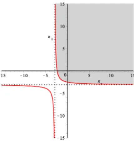
(10) 66. The. precise forms of A^{D},. the form of A^{D} :. B_{\pm}^{D}. ,. and C^{D}. are. obtained. by using Maple 17. Here,. we. show. only. A^{D}(H_{*}^{+}, B, d, $\tau$). =\displaystyle \frac{1}{8(H_{*}^{+})^{3}PQ}[(H_{*}^{+})^{2}(1-B^{2})^{2}I_{1}^{2}\cos(2H_{*}^{+} $\tau$)\cos(2H_{*}^{+}(d- $\tau$)) -4(H_{*}^{+})^{2}(1+B^{2})I_{1}I_{2}\cos(2H_{*}^{+} $\tau$)\cos(2H_{*}^{+}(d- $\tau$)). +3(H_{*}^{+})^{2}I_{2}^{2}\cos(2H_{*}^{+} $\tau$)\cos(2H_{*}^{+}(d- $\tau$)). +2H_{*}^{+}(1+B^{2})I_{1}\{P\sin(2H_{*}^{+} $\tau$)\cos(2H_{*}^{+}(d- $\tau$))+Q\cos(2H_{*}^{+} $\tau$) sin (2H_{*}^{+}(d- $\tau$ -4H_{*}^{+}BI_{1}\{P\cos(2H_{*}^{+}(d- $\tau$))-Q\cos(2H_{*}^{+} $\tau$)\} -4H_{*}^{+}I_{2}\{P\sin(2H_{*}^{+} $\tau$)\cos(2H_{*}^{+}(d- $\tau$))+Q\cos(2H_{*}^{+} $\tau$)\sin(2H_{*}^{+}(d- $\tau$ +2PQ\{1+\sin(2H_{*}^{+} $\tau$)\sin(2H_{*}^{+}(d- $\tau$ -(P^{2}+Q^{2})\cos(2H_{*}^{+} $\tau$)\cos(2H_{*}^{+}(d- $\tau$. ,. where. P(H_{*}^{+}, B, $\tau$)=\sqrt{1+B^{2}-2B\sin(2H_{*}^{+} $\tau$)}, Q(H_{*}^{+}, B, d, $\tau$)=\sqrt{1+B^{2}+2B\sin(2H_{*}^{+}(d- $\tau$} Moreover, by. the. help. with. Maple 17,. we. have. B_{-}^{D}(H_{*}^{+}, i, d, $\tau,\ \theta$_{+})B_{+}^{D}(H_{*}^{+}, B, d, $\tau,\ \theta$_{-})-A^{D}(H_{*}^{+}, B, d, $\tau$)C^{D}(H_{*}^{+}, B, d, $\tau,\ \theta$_{+}, $\theta$_{-}). =\displaystyle \frac{1}{16(H_{*}^{+})^{4}PQ}[H_{*}^{+}\{(1+B^{2})(1+\sin(2H_{*}^{+} $\tau$)\sin(2H_{*}^{+}(d- $\tau$ -(P^{2}+Q^{2})\}I_{1} +H_{*}^{+}(3-\sin(2H_{*}^{+}(d- $\tau$))\sin(2H_{*}^{+} $\tau$))I_{2}. -P\cos(2H_{*}^{+} $\tau$)\sin(2H_{*}^{+}(d- $\tau$))-Q\sin(2H_{*}^{+} $\tau$)\cos(2H_{*}^{+}(d- $\tau$))]^{2}\geq 0.. Theorem 3.1 Set. D($\kappa$_{\mathrm{I}\mathrm{I}\pm)}H_{*}^{+}, B, d, $\tau,\ \theta$_{\pm}). :=A^{D} (H_{*}^{+}, B, d, $\tau$)$\kappa$_{\mathrm{I}\mathrm{I}_{-} $\kappa$_{$\Pi$_{+} +B_{-}^{D}(H_{*}^{+}, B, d, $\tau,\ \theta$_{+})$\kappa$_{$\Pi$_{-} +B_{+}^{D}(H_{*}^{+}, B, d, $\tau,\ \theta$_{-})$\kappa$_{\mathrm{I}\mathrm{I}+} +C^{D}(H_{*}^{+}, B, d, $\tau,\ \theta$_{+}, $\theta$ H_{*}^{+}d. and let q_{1} be the value of $\kap a$_{\mathrm{I}\mathrm{I}\pm},. which is the 1st. zero‐point of A^{D}. .. If the parameters. H_{*}^{+}, B, d, $\tau$, $\theta$_{\pm} satisfy \hat{D}. then the. ($\kap a$_{$\Pi$_{\pm} , H_{*}^{+}, B, d, $\tau,\ \theta$_{\pm})>0,. Delaunay surfaces. Theorem 3.2 If. surfaces. are. H_{*}^{+}d. stable.. are. $\kap a$_{\mathrm{I}\mathrm{I}_{-}. linearly. stable under. \geq q_{1} then there ,. >-\displaystyle\frac{B_{+}^{D}(H_{*}^{+},Bd,$\tau,\theta$_{-}) {A^{D}(H_{*}^{+},Bd,$\tau$)}. are no. an. pairs of. ,. and. H_{*}^{+}d<q_{1}. ,. (16). axisymmetric perturbation.. ($\kap a$_{\mathrm{I}\mathrm{I}_{-} , $\kap a$_{\mathrm{I}\mathrm{I}+}). such that the. Delaunay.

(11) 67. H_{*}^{+}d\approx 1.6348. H_{*}^{+}d\approx 2.4759 A part of unduloids. H_{*}^{+}d\approx 4.7764. (B=0.75). .. H_{*}^{+}d\approx 1.3089 H_{*}^{+}d\approx 1.2720 A part of nodoid (B=1.05) sphere.. A part of. Figure. 6: The. Delaunay surfaces with. $\theta$_{-}=\displaystyle\frac{$\pi$}{4}. and. .. $\theta$_{+}=\displaystyle\frac{$\pi$}{3}.. Examples. 4. Concerning. $\pi$/2. ,. see. criteria of. [10, 11].. given by Fig.. stability. for. In this paper,. cylinders. we. and unduloids with. consider the. stability. of. $\tau$= $\pi$/(4H_{*}^{+}). unduloids, sphere,. under. $\theta$\pm. =. and nodoid. 6.. For unduloids in this setting, we can obtain q_{1}\approx 2.6310 by the help with Maple 17. Thus, by Theorem 3.2, the unduloid with H_{*}^{+}d\approx 4.7764 is unstable. In the cases H_{*}^{+}d\approx 1.6348 and H_{*}^{+}d\approx 2.4759 the criteria of the unduloids are given by Fig. 7. By Theorem 3.1, unduloids are stable under an axisymmetric perturbation, provided that ($\kap a$_{\mathrm{I}\mathrm{I}_{-} , $\kap a$_{ $\Gam a$ \mathrm{I}+}) is included in the in 7. is For gray parts Fig. H_{*}^{+}d\approx 1.6348, ($\kappa$_{$\Pi$_{-} , $\kappa$_{\mathrm{I}\mathrm{I}+})=(0,0) included in the gray part, so that the unduloid with H_{*}^{+}d\approx 1.6348 is stable under an axisymmetric perturbation. On the other hand, for H_{*}^{+}d\approx 2.4759, ($\kappa$_{\mathrm{I}\mathrm{I}_{-} , $\kappa$_{$\Pi$_{+} )=(0,0) is not included in the gray part. Thus the ,. unduloid with For. sphere. H_{*}^{+}d\approx 2.4759 in this. is unstable.. setting,. we. consider the. problem. in the interval. [0. ,. 2.3561 ]. .. In this.

(12) 68. H_{*}^{+}d\approx 1.6348 H_{*}^{+}d\approx 2.4759 Figure. 7: The criteria of unduloids with. Figure. 8: The criterion of the. H_{*}^{+}d=1.6348. sphere. with. and. H_{*}^{+}d\approx 2.4759.. H_{*}^{+}d\approx 1.3089..

(13) 69. Figure. 9: The criterion of the nodoid with. H_{*}^{+}d\approx 1.2720.. interval, wc havc no value of H_{*}^{+}d which is the zero‐point of A^{D} Thus we can jude the stability by using Fig. 8. ($\kappa$_{$\Pi$_{-}}, $\kappa$_{$\Pi$_{+}})=(0,0) is included in the gray part, so that the sphere with H_{*}^{+}d\approx 1.3089 is stable under an axisymmetric perturbation. For nodoid in this setting, we can obtain q_{1} \approx 2.3389 by thc help with Maplc 17. Thc criterion of the nodoid with H_{*}^{+}d\approx 1.2720 is given by Fig. 9. Then we see that ($\kappa$_{$\Pi$_{-} , $\kappa$_{$\Pi$_{+} )= .. (0,0). H_{*}^{+}d\approx. is included in the gray part. Thus the nodoid with. 12720 is stable under. an. axisymmetric perturbation.. Acknowledgements This work was supported by JSPS 24244012, 25247008.. KAKENHI Grant Numbers. 24540200,. References [1]. H.. Abels,. mean. [2]. M.. [3]. A. J.. R. Courant and D.. D.. mean. curvature. surfaces. free. Hilbert,. Methods. of. mathematical. physics, vol.I, Interscience,. New. 1953.. Depner, Linearized stability analysis of surface diffusion for hypersurfaces contact, Math. Nachr., 285 (2012), no. 11‐12, 1385‐1403.. ary. with. Bernoff, A. L. Bertozzi, T. P. Witelski, Axisymmetric surface diffusion: dynamics stability of self‐similar pinchoff, J. Statist. Phyb 93 (1998), no. 3‐4, 725‐776.. York,. [5]. Garcke, and L. Müllcr, Stability of spherical caps under the volume‐preserving flow with line tension, Nonlinear Anal., 117 (2015), 8‐37.. Athanassenas, A variational problem for constant boundary, J. Reine Angew. Math., 377 (1987), 97‐107.. and. [4]. H.. curvature. with bound‐.

(14) 70. [6]. L. G. Fel and B. Y. 66. Phys.,. [7]. R.. [8]. H.. (2015),. Rubinstein, Stability of axisymmetric liquid bridges, 6, 3447‐3471.. Equilibrium Capillary Surfaces, Springer New York, 1986.. Finn,. Z.. Angew. Math.. Issue. Grundlehren. der. mathematischen. Wis‐. senschaften 284,. K. Ito, and Y. Kohsaka, Surface diffusion with triple junctions: a stability for stationary solutions, Adv. Differential Equations, 15 (2010), no. 5‐6, 437−. Garcke,. creterion. 472.. [9]. [10]. [11] [12]. Kenmotsu, Surfaces with Monographs, AMS, 2003.. Constant Mean. Katsuei. ical. Curvature, Translations of Mathemat‐. Kohsaka, Stability analysis of Delaunay surfaces as steady states for the sur‐ face diffusion equation, Geometric Properties for Parabolic and Elliptic PDEs, Springer Proceedings in Mathematics & Statistics 176, 121‐148, Springer International Publishing Switzerland, 2016. Yoshihito. Yoshihito. Kohsaka, On. the criteria. Kôkyûroku. Bessatsu B63. (2017),. J.. for. the. stability of unduloids,. To appear in RIMS. 167‐192.. LcCrone, G. Simonett, On well‐posedness, stability, and bifurcation for the axisym‐ surface diffusion flow, SIAM J. Math. Anal., 45 (2013), no. 5, 2834‐2869.. metric. [13] [14]. A. D. Myshkis, V. G. Babskii, N. D. Kopachevskii, L. A. Slobozhanin, and A. Tyuptsov, Low‐Gravity Fluid Mechanics, Springer‐Verlag Berlin Heidelberg, 1987. B. Y. Rubinstein and L. G. two solid. [15] [16]. Fel, Stability of unduloidal and nodoidal spheres, J. Geom. Symmetry Phys., 39 (2015), 77‐98.. Vogel, Stability of a liquid drop trapped between Math., 47 (1987), no. 3, 516‐525. T. I.. T. I.. Vogel, Stability of a liquid drop trapped angles, SIAM J. Appl. Math., 49 (198g). contact. [17]. T. I.. Math.,. [18] [19]. two. (2006),. no.. menisci between. parallel planes, SIAM. no.. between. spheres, Pacific J.. 2, 367‐377. Math. Fluid. Vogel, Liquid Bridges between Contacting Balls, J. Math. Fluid Mech.,. 737‐744.. [20J. Appl.. parallel planes. II. General 4, 1009‐1028.. T. I. Vogel, Liquid Bridges Between Balls: The Small Volume Instability, J. Mech., 15 (2013)} no. 2, 397‐413. T. I.. J.. between two ,. Vogel, Convex_{J} rotationally symmetric liquid bridges 224. D.. S. Yotsutani and M. Murai, \mathrm{F}_{\mathrm{F}\exist }\mathrm{N}\ovalbox{\t \smal REJECT} \mathscr{X}\mathrm{E}\'{I}_{1}\mathrm{f}:\mathrm{E} \langle. $\gamma$_{\grave{*}65}, \mathrm{B}*\neg\vec{i\vec{-} +r\vec{\frac{} \simeq $\beta$} \# 7\pm. ,. 2013.. 16. (2014),.

(15)