Bifurcation analysis of an equation
for gas discharge
鈴木政尋
MASAHIRO SUZUKI *名古屋工業大学大学院工学研究科
GRADUATE SCHOOL OF ENGINEERING,NATOYA INSTITUTE OF TECHNOLOGY
1 Introduction
The main purpose of this paper is to analyze mathematically the fundamental mech‐ anism of gas ionization processes. Nowadays plasmas are widely applied in various fields such as environmental improvement and engineering. The environmental applications are the production of ozone from air with water cleaning and the elimination of biologi‐ cal contamination. Engineers use plasma for material processing and surface deposition, electromagnetic absorbers and reflectors, and so on. Therefore, interest in the study of plasma generation has been increasing.
Townsend discovered the fundamental mechanism of gas ionization around 1900. He experimented and considered what happens in a chamber formed from two planar parallel plates and filled with a gas when a direct current high‐voltage is applied between these two plates. Here the lower voltage plate is the cathode, and another one is the anode. As a consequence, it was observed that there are two mechanisms for a gas ionization
process. If electrons are emitted by irradiation of\mathrm{X}‐rays to the cathode, these initial elec‐
trons are accelerated from the cathode to the anode by high‐voltage and simultaneously make ions and additional electrons owing to the collision of electrons with gas particles.
This mechanism is called as $\alpha$‐mechanism. Another mechanism, called as $\gamma$‐mechanism,
is the secondary emission of electrons caused by impact of positive ions with the cathode. If applied voltage is sufficiently high, these two mechamisms lead to the electric multipli‐ cation which permit large current flow throughout the gas which is an insulator. This phenomenon is called as avalanche breakdown or gas discharge. Townsend also derived a
threshold of voltage at which gas discharge happens continuously. The threshold is called as sparking voltage. In this process, he used several simplification such as discretization
of time, ignorance of advection, and so on (for more details, see [14]). Hence, it is an in‐
teresting problem to analyze the sparking voltage by using a partial differential equation with no simplification.
Morrow derived the mathematical model in [11]. After that, several models were proposed and used in [1, 5, 6, 7, 8, 9]. These models vary with the constitutive equations
of velocities. On the other hand, Degond and Lucquin‐Desreux in 2007 gave the formal
derivation of the model, derived by Morrow, from the Euler‐Maxwell equations (see [4]).
At this point, it seems reasonable to analyze this model. In this paper, we call it as the Degond−Lucquin‐Desreux−Morrow model. It consists of two continuity equations for the densities of positive ions and of electrons, adopting constitutive velocity relations, coupled with the Poisson equation for the electrostatic potential:
\partial_{t}$\rho$_{i}+\partial_{x}($\rho$_{i}u_{i})=a\exp(-b|\partial_{x} $\Phi$|^{-1})p_{e}|v_{e}|
, (1a)\partial_{t}$\rho$_{e}+\partial_{x}($\rho$_{e}v_{e})-k_{e}\partial_{xx}$\rho$_{e}=a\exp(-b|\partial_{x} $\Phi$|^{-1})$\rho$_{e}|v_{e}|
, (1b)$\lambda$\partial_{xx} $\Phi$=$\rho$_{i}-$\rho$_{e}. (1c)
v_{e}:=-k_{e}\partial_{x} $\Phi$, u_{i}:=k_{i}\partial_{x} $\Phi$. (1d)
The unknown functions $\rho$_{i}, p_{e}, and - $\Phi$ denote the positive ion density, the electron
density, and the electrostatic potential, respectively. The ion and electron velocities u_{i}
and u_{e} are assumed to obey (1d). Moreover, k_{i}, k_{e}, a, b, and $\lambda$ are positive constants. The right hand sides of (1a) and (1b) come from $\alpha$‐mechanism. In particular, $\alpha$ =
aexp
(-b|\partial_{x} $\Phi$|^{-1})
is the first Townsend ionization coefficient expressing the number of ion‐electron pairs generated per unit volume by the electron impact ionization. We notice that this model is a hyperbolic‐parabolic‐elliptic coupled system by substituting constitutive
velocity relations (1d) into continuity equations (1a) and (1b).
We consider the initial‐boundary value problem of this model over the bounded in‐
tervalI:=(0, L) by prescribing the initial and boundary data
($\rho$_{i}, $\rho$_{e})(0, x)=($\rho$_{i0}, $\rho$_{e0})(x) , $\rho$_{i0}(x)\geq 0, $\rho$_{e0}(x)\geq 0, x\in I, (1e)
$\rho$_{i}(t, 0)=$\rho$_{e}(t, 0)= $\Phi$(t, 0)=0, (1f)
$\rho$_{e}(t, L)=0, $\Phi$(t, L)=V_{c}>0. (\mathrm{l}\mathrm{g})
The boundariesx=0andx=Lcorrespond to the anode and cathode, respectively, since
- $\Phi$ is the electrostatic potential. Boundary condition (1f) means that, in an instant,
electrons are absorbed to the anode and ions are excluded near the anode. We emphasize
that $\gamma$‐mechanism is not taken into account on the cathode x = L, and thus the zero
assume the non‐negativity of initial densities $\rho$_{i0} and $\rho$_{e0}. For the compatibility, we let
the initial dataR_{i0} andR_{e0} satisfy
R_{i0}(0)=R_{e0}(0)=R_{\mathrm{e}0}(\mathrm{L})=0.
For the Degond−Lucquin‐Desreux−Morrow model and the related models, there are a
lot of numerical researches (for example, see [10, 12, 13 On the other hand, only two
mathematical results for this model has been announced by the authors. The first result
[15] established a mathematical framework for analyzing this model rigorously. More
precisely, they showed the time‐local solvability of the initial boumdary value problem
over a domain $\Omega$
:=\mathbb{R}_{+}^{3}\backslash K
, where\mathbb{R}_{+}^{3}
is a half space, Kis a simply connected open set,and the intersection of
\partial \mathbb{R}_{+}^{3}
and Kis the empty set. The second result [16] investigated the sparking voltage, which is required when gas discharge happens continuously, by using(1). Specifically, the authors analyzed the bifurcation of the stationary solutions to (1)
and then concluded that gas discharge may happen even for the no $\gamma$‐mechanism case.
This conclusion essentially differs from Townsend theory, since his theory explains that
no gas discharge happens if there is no $\gamma$‐mechanism. In this short paper, we review this
bifurcation analysis. Before closing this section, we give a notation.
Notation For 1\leq p\leq\infty,L^{p}( $\Omega$)is the Lebesgue space equipped with the norm |\cdot|_{p}. For
a non‐negative integerk,
H^{k}(I)
is the k‐th order Sobolev space inL^{2}sense, equipped withthe norm \Vert\cdot\Vert_{k}. Moreover,
H_{0}^{1}(I)
andH_{0l}^{1}(I)
are closures ofC_{0}^{\infty}(I) andC_{0}^{\infty}((0, L]) withrespect to H^{1}‐norm, respectively. We denote by C^{m}([0, T];X) the space of the m‐times
continuously differentiable functions on the interval [0, T] with values in a Banach space
X, and by H^{m}(0, T;X) the space of H^{m}‐fUnctions on (0, T) with values in a Banach
space X.
2 Main results
For mathematical convenience, let us rewrite initial‐boundary value problem (1) by
using the new unknown functions
R_{ $\eta$}\cdot:=$\rho$_{i}e^{-\frac{L}{V_{\mathrm{C}}}x}, R_{e}:=$\rho$_{e}e^{V}\vec{2L}x
and the new given functions
h(x):=aexp
(\displaystyle \frac{-b}{|x|})|x|, g(V_{c}):=h(\displaystyle \frac{V_{c}}{L})
-\displaystyle \frac{V_{c}^{2}}{4L^{2}}.
Furthermore, we also decompose the electrostatic potential‘aswhereV_{c}x/Lis a solution to the equation\partial_{xx}u=0with the boundary conditions u(0)=0
andu(L)=V_{c}. As a result, we have the following rewritten problem
\displaystyle \partial_{t}R_{i}+k_{i}\partial_{x}\{(\partial_{x}V+\frac{V_{c}}{L})R_{\dot{ $\eta$}}\}+k_{i}R_{\dot{ $\eta$}}=k_{e}h(\frac{V_{\mathrm{c}}}{L})e^{-\frac{L}{V_{\mathrm{c}}}x_{\vec{2L}}^{V}x}-R_{e}+k_{i}f_{i}
, (2a) \partial_{t}R_{e}-k_{e}\partial_{xx}R_{e}-k_{e}g(V_{c})R_{e}=k_{e}f_{e}, (2b)V[R_{ $\eta$}\displaystyle \cdot, R_{e}]:=\frac{1}{ $\lambda$}\int_{0}^{L}G(x, y)
(
e^{\frac{L}{V_{\mathrm{c}}}y}
瓦
(t, y)-e^{-\rightharpoonup y}2VLR_{e}(t, y)
)
dy,
(2c)
(R_{ $\eta$}\cdot, R_{e})(0, x)=(R_{ $\eta$ 0}, R_{e0})(x) , R_{\dot{ $\eta$}0}(x)\geq 0, R_{e0}(x)\geq 0, (2d)
R_{ $\eta$}\cdot(t, 0)=R_{e}(t, 0)=R_{e}(t, L)=0, (2e)
where G(x, y) is the Green function of the Laplace operator with the Dirichlet zero con‐
dition, and the nonlinear terms f_{i} and f_{\mathrm{e}} are defined as
f_{i}:=-R_{ $\eta$}\displaystyle \cdot\partial_{x}V-\frac{k_{e}}{k_{i}}\{h(\frac{V_{c}}{L}) -h(\partial_{x}V+\frac{V_{c}}{L})\}e^{-\frac{L}{V_{c}}x_{2L}^{V}x}-\rightharpoonup R_{e},
f_{e} :=\displaystyle \partial_{x}V\partial_{x}R_{e}-\frac{V_{\mathrm{c}}}{2L}R_{e}\partial_{x}V+R_{e}\partial_{xx}V-\{h(\frac{V_{c}}{L}) -h(\partial_{x}V+\frac{V_{c}}{L})\}R_{e}.
It is easy to check that the corresponding stationary problem has a trivial stationary solution
(鳥,R_{e}) =(0,0) .
The advantage of using the new known functions R_{\dot{ $\eta$}} and R_{e} lies in the following two
facts. The first one is that the rewritten hyperbolic equation has the dissipative term
k_{i}R_{\dot{ $\eta$}}, although the original hyperbolic equation does not have any dissipative structure.
Secondly, the linear part of the rewritten parabolic equation is self‐adjoint. These two facts play important roles in the proofs of both the nonlinear stability and instability of the trivial stationary solution.
We are now in a position to state the stability and instabihty theorems for the trivial
solution.
Theorem 1. Let g(V_{c}) <
$\pi$^{2}/L^{2}
. There exists $\epsilon$ > 0 such that if the initial data(R_{ $\eta$ 0}, R_{e0}) \in
H_{0l}^{1}
\timesH_{0}^{1}
satisfies \Vert R_{n0}\Vert_{1} + \Vert R_{e0}\Vert_{1} < $\epsilon$, then problem (2) has a uniquetime global solution (R_{\mathrm{h}}, R_{e}) as
凡 \geq 0, 鳥
\in C([0, \infty);H_{0l}^{1})\cap C^{1}([0, \infty);L^{2})
, (3a)R_{e}\geq 0, R_{e}\in C([0, \infty);H_{0}^{1})\cap L^{2}(0, \infty;H^{2})\cap H^{1}(0, \infty;L^{2})
. (3b)Moreover, it converges to zero exponentially fast in H^{1}\times H^{1} astgoes to infinity.
Theorem 2. Let
g(V_{c})>$\pi$^{2}/L^{2}
and($\psi$_{i}, $\psi$_{e})\in H_{0l}^{1}\times H_{0}^{1}
satisfyThere exists $\varepsilon$ > 0 such that for any sufficiently small $\delta$ > 0, problem (2) with the
initial data (R_{ $\eta$ 0}, R_{e0}) = ( $\delta \psi$_{i}, $\delta \psi$_{e}) has a unique solution (R_{i}, R_{e}) satisfying \Vert R_{i}(T)\Vert_{1}+
\Vert R_{e}(T)\Vert_{1}\geq $\varepsilon$for some T>0.
In this instability theorem, the last inequality in (4) is equivalent to that the initial data R_{e0} is a non‐zero function. One may ask what happens for the case that R_{e0} is the zero function. Proposition 3 gives the answer that there exists a unique time global solution, and it attains the trivial stationary solution at finite time.
Proposition 3. LetV_{c}>0. There exists $\epsilon$>0 such that if the initial data (R_{\dot{n}0}, R_{e0}) \in
H_{0l}^{1} \times H_{0}^{1}
satisfies R_{e0} = 0 and \Vert R_{n0}\Vert_{1} < $\varepsilon$, then problem (2) has a unique time globalsolution (R_{ $\eta$}\cdot, R_{e}) as (3). Furthermore, there existsT_{0}>0 such that
(R_{ $\eta$}\cdot, R_{e})(t, x)=(0,0) for (t, x)\in[T_{0}, \infty) \times I. (5)
Remark 4. This proposition asserts that a set
\{(R_{n0}, R_{e0}) \in H_{0l}^{1} \times H_{0}^{1}; R_{e0} = 0\}
is alocal stable manifold of system (2\mathrm{a})-(2\mathrm{c}) for anyV_{c}>0.
We can expect from Crandall and Rabinowitz’s Theorem (see [2, 3 and Theorems 1
and 2 by regarding the voltage V_{c}as the bifurcation parameter that there is a non‐trivial
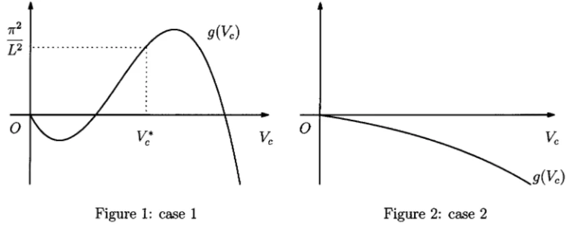
solution curve near the point (R_{ $\eta$}\cdot, R_{e}, V_{c})=(0,0, V_{c}^{*}), where V_{c}^{*} is defined as
g(V_{c}^{*})=\displaystyle \frac{$\pi$^{2}}{L^{2}}, g'(V_{c}^{*})>0
. (6)It is straightforward to check that the graph of the functiong is drown as Figures 1 and
2, where there exists two cases subject to the physical parameters a, b, and L. For the
first case as Figure 1, it has one local minimum and one global maximum. For the second case as Figure 2, it is strictly decreasing. Note that both cases are truly possible. We
study only the first case hereafter and thus see that V_{\mathrm{c}}^{*} in (6) is well‐defined.
\mathrm{c}
Figure 1: case 1
)
Figure 2: case 2 The bifurcation results are summarized in Theorem 5 and Corollary 6.
Theorem 5. For V_{c}^{*} defined in (6), there exist $\eta$ > 0, V_{c} \in
C^{2}([- $\eta$, $\eta$];\mathbb{R})
, and z \inC^{2}([- $\eta$, $\eta$];H^{1}\times H^{2})
such thatV_{\mathrm{c}}(0)=V_{c}^{*}, z(0)=0, and stationary problem to (2) withV_{c}=V_{c}(s) has a non‐trivial solution(R_{ $\eta$}\cdot, R_{e})(s)=s($\varphi$_{i}, $\varphi$_{e})+sz(s) fors\in[- $\eta$, $\eta$], where
$\varphi$_{i}(x) :=\displaystyle \frac{k_{e}}{k_{i}}\exp(\frac{-bL}{V_{c}^{*}})e^{-\frac{L}{V_{c}^{*}}x}\int \mathrm{o}^{x*}e^{-\frac{V}{2}c_{-y}}L$\varphi$_{e}(y)dy, $\varphi$_{e}(x) :=\sin\frac{ $\pi$}{L}x.
Moreover,
\dot{V}_{c}(0)>\leq 0
holds if and only if-Lg'(V_{\mathrm{c}}^{*})\displaystyle \int_{0}^{L}$\varphi$_{e}^{2}\partial_{x}V[$\varphi$_{i}, $\varphi$_{e}]dx-\frac{1}{2}\int_{0}^{L}$\varphi$_{e}^{2}\partial_{xx}V[$\varphi$_{i}, $\varphi$_{\mathrm{e}}]dx\leq 0>.
Corollary 6. Let
\dot{V}_{c}(0)\neq 0
. For s\neq 0, it holds for anyx\in(0, L) thats\dot{V}_{c}(0)R_{ $\eta$}\cdot(s)>0, s\dot{V}_{c}(0)R_{e}(s)>0.
Furthermore, the positive non‐trivial solution is linearly stable if
\dot{V}_{c}(0)
> 0, and thepositive non‐trivial solution is linearly unstable if
\dot{V}_{c}(0)<0.
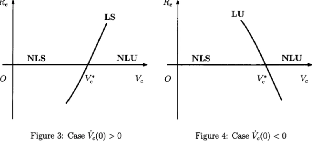
From Theorem 5 and Corollary 6, we can draw the bifurcation diagram of stationary solutions as Figures 3 and 4. The both diagrams are truly possible for some physical
parameters k_{i}, k_{e}, a, b, and L. For example, one can have
\dot{V}_{c}(0)
> 0 by letting k_{e}/k_{i}sufficiently small; one can have
\dot{V}_{c}(0)<0
by letting k_{e}/k_{i} sufficiently large and assumingan additional condition fora, b, and L.
Figure 3: Case
\dot{V}_{c}(0)>0
Figure 4: Case\dot{V}_{c}(0)<0
Let us mention physical observation from the above bifurcation analysis. Townsend defined the sparking voltage as a threshold of voltage at which gas discharge happens continuously. In the following his manner, it is reasonable to define the sparking voltage for
the solution to this model may approach to the positive non‐trivial stationary solution
as t tends to infinity if
\dot{V}_{\mathrm{c}}(0)
> 0; the solution may either blow up or grow up as timegoes by if
\dot{V}_{c}(0)
< 0. Hence, the solution never goes to the trivial stationary solution(R_{ $\eta$}\cdot, R_{e})=(0,0). On the other hand, for the case V_{c}<V_{c}^{*}, the solution converges to the
trivial solution asttends to infinity. These facts mean that V_{c}^{*} is a threshold of voltage at
which gas discharge happens continuously from physical point of view. Therefore we can
conclude that gas discharge can happen even if $\gamma$‐mechanism is not taken into account,
whereas it cannot happen without $\gamma$‐mechanism in Townsend theory.
Acknowledgments This result is obtained through the joint research with Prof. Atusi Tani at Keio University.
References
[1] I. Abbas and P. Bayle, A critical analysis of ionising wave propagation mechanisms
in breakdown, J. Phys. D: Appl. Phys. 13 (1980), 1055‐1068.
[2] M. Crandall and P. H. Rabinowitz, Bifurcation from simple eigenvalues, J. Func‐
tional Analysis 81971321‐340.
[3] M. Crandall and P. H. Rabinowitz, Bifurcation, perturbation of simple eigenvalues and linearized stability, Arch. Ration. Mech. Anal. 52 (1973), 161‐180.
[4] P. Degond and B. Lucquin‐Desreux, Mathematical models of electrical discharges in
air at atmospheric pressure: a derivation from asymptotic analysis, Int. J. Compu.
Sci. Math. 1 (2007), 58‐97.
[5] S. K. Dhali and P. F. Williams, Twodimensional studies of streamers in gases, J.
Appl. Phys. 62 (1987), 4694‐4707.
[6] P. A. Durbint and L. Turyn, Analysis of the positive DC corona between coaxial
cylinders, J. Phys. D: Appl. Phys. 20 (1987), 1490‐1496.
[7] A. A. Kulikovsky, Positive streamer between parallel plate electrodes in atmospheric pressure air, IEEE Trans. Plasma Sci. 30 (1997), 441‐450.
[8] A. A. Kulikovsky, The role of photoionization in positive streamer dynamics, J.
Phys. D: Appl. Phys. 33 (2000), 1514‐1524.
[9] A. Luque, V. Ratushnaya and U. Ebert, Positive and negative streamers in ambient
air: modeling evolution and velocities, J. Phys. D: Appl. Phys. 41 (2008), 234005.
[10] J.‐C. Mateéo‐Vélez, P. Degond, F. Rogier, A. Séraudie and F. Thivet, Modelling wire‐
to‐wire corona discharge action on aerodynamics and comparison with experiment,
[11] R. Morrow, Theory of negative corona in oxygen, Phys. Rev. A 32 (1985), 1799‐1809.
[12] R. Morrow, The theory of positive glow corona, J. Phys. D: Appl. Phys. 30 (1997),
3093‐3114.
[13] R. Morrow and J. J. Lowke, Streamer propagation in air, J. Phys. D: Appl. Phys.
30 (1997), 614‐627.
[14] Y. P. Raizer, Gas Discharge Physics, Springer, 2001.
[15] M. Suzuki and A. Tani, Time‐local solvability of the Degond‐Lucquin‐Desreux‐
Morrow model for gas discharge, submitted.
[16] M. Suzuki and A. Tani, Bifurcation analysis of the Degond−Lucquin‐Desreux−Morrow