Finely-tuned Plots in LATEX for Statistics Education utilizing an R-based KETpic Plug-In (Computer Algebra Systems and Education : A research about Effective Use of CAS in Mathematics Education)

Finely-tuned

Plots

in

_LATEX

for

Statistics Education

utilizing

an

R-based

KETpic

Plug-In

Shunji Ouchi

Economics

Shimonoseki

City University

Setsuo

Takato

Pharmaceutical

Sciences

Toho University

Abstract

We have been developing $I\Phi r_{P}ic$ as alibrary ofmacro package of Computer Algebra

Systems(CAS) to generatestandard

_IATffi

sourcecode for high-quality scientific artwork.

We have recently implemented $I\Phi r_{pic}$ in $R$, which is a popular open-source software

tool used in statistical analysis and for graphic output. It is often the case that the

default or standard output from $R$ is not exactly what the users requires, particularly

when producing graphics for educational purposes. Through taking full advantage of the

functionality of$R$ and IATffl, $I\Phi r_{P}ic$ enables us to produce teaching/learning materials

incorporating figures which aredesigned to help the leamer better understand statistical

ideas and theories. In this paper we look at the use ofthe plug-in to generate two basic statistical plots, the histogram andboxplot, whicharemost useful in descriptive statistics.

We will also describe $I\Phi r_{P}ic$ functionality that can be usedto produce enhanced graphic

output.

1

Introduction

According to a recent survey conducted by the authors in Japan[l], about 74 percent from a

sample of 378 who teach mathematics to first and second-year university or technical college

students utilise $IA^{r}I\varpi$to create teaching/learning materials. Nowadays 聾丁回(is particularly

valuableforuniversityandcollegemathematicsteachersas atoolforpreparing printedmaterials

in Japan.

When teachers want to include graphics into a $I4Tffi$ document, most of them will do so

using data formatted as EPS files. These files are then inserted into the $I\#Tffl$ text file using

the ‘includegraphics’ command. However, this method has some disadvantages. There are

a number of reasons for this: the size of the EPS file is not small; the canvas dimension of

the graphic is not easily handled; and the graphics embbedded in the

_IAEX

file is difficult to

fine-tune. What $RT\varpi$ actually provides is very limited set of graphical capabilities to yield

drawings.

On the other hand our $Iqr_{P}ic$ plug-in, finely-tuned control of various graphical features

such

as

line style, shading, and text display is enabled until the

user

$s$ needs are fully satisfied.

R-based $Iqr_{P}ic$ commands allow us to convert graphic outputs of $R$ into Tpic specials

easily produce ]_{$yIffi$ documments incorporating figures which are designed to help the learner}

better understand statistical ideas and theories using $I\Phi r_{P}ic$.

In this paper we look at the use of R-based $I\Phi r_{pic}$ plug-in to enhance standard statistical

graphic output of $R$ in

BTffi

andsome interesting _{$Iqr_{pic}$} capabilities are discussed by means

of illustrative examples.

2

$R$

and Its

Graphic Output

$R$ is a popular open-source software environment licenced under the GNU General Public

Licence used in statistical computing and production of graphics. It provides a wide variety

of statistical and graphical techniques, and is highly extensible. $R$ compiles and

runs

on a

wide variety ofplatforms, such as Windows, the Macintosh operating system and UNIX. The

software can be obtained from the Comprehensive R Archive Network (CRAN) accessible via

the main $R$ web site http:$//ww$

.

r-project.org.

In $R$ functions the graphics systems and graphics packages can be divided into three main

types: high-level functions that produce complete plots; low-level functions that add further

output to

an

existing plot; and functions for working interactively with graphical output (see

[7]$)$. The main high-level plotting functions are the ones used to produce complete plots such

as scatterplots, histograms, and boxplots.

Here we demonstrate simple usage of high-level and low-level functions in $R$ session.

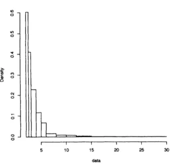
Pro-ducing a histogram using high-level function hist is done by:

cl $<-c(2,2.5,3,4,5.6,8.10,12,15,20.25,30)$

hist(data,breaks$=c1$) $\#$ ‘data’ is data set

with the output as seen in Figure 1.

$H|\cdot|0\mathfrak{g}ram$ofdata

$0$

5 10 15 20 25 30

data

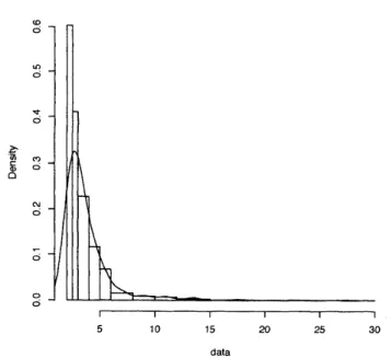
Next we add a density estimate tothe existing graphic using low-levelfunction Iines.

lines (density(data))

$\#$ The density function finds a density estimate

from the data

giving us the graph below (Figure 2).

Histogram ofdata

$\overline{5101520253}0$

data

Figure 2 Graphic output of histogram with density estimate

3

Flow of

$I\Phi r_{P}ic$

drawing

Figure 3 illustrates the $Iqr_{P}ic$ Graphical Pipeline for R.

Figure 3 $I\mathfrak{g}FPiC$ graphical pipeline for $R$

We will demonstrate the $Iqr_{P}ic$ session workflow by outlining of process of enhancing the

Figure 4, $Iqr_{P}ic$ enable us to achieve this aim. While $R$ itself is equipped with some basic

commands or functions for modifying the standard graphic output, it doesn $t$ include powerful

features users demand.

Often

to obtain high-quality graphics,

users

must work with the

R-created graphics in a third-party graphical editor such as Adobe Illustrator. $Iw_{P}ic$ provides

an economical alternative to this, and also has lower requirements producingsmaller sized files

than the EPS format files researchers often need to work with.

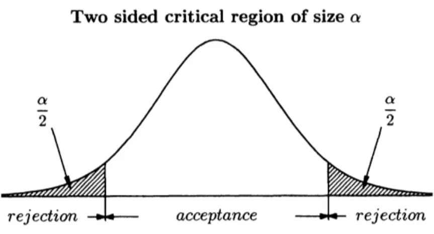
Two sided critical region ofsize $\alpha$

Figure 4 Graphic output of$Iqr_{P}ic$

The user begins by opening $R$ for anew session. We start by loading the plug in:

load$(^{t1}ketpic$

.

Rdata“)

This is an important step as it ensures all new $I\Phi r_{P}ic$ commands are automatically available

from the very beginning.

step I Aftersettingup thecanvas dimensions for$I4^{r}Iffl$drawing, theuser runs$R$commands,

routines and libraries to perform computations and generategraphic output.

Setwindow$(c(-3,3), c(-0.1,0.41))$

Setscaling(6.46)

Gl $<$-Plotdata$(^{1t}dt(x, 10)$“,“$x^{t1}$,“$N=100$“$)$

G2 $<$-Listplot($c$(XMIN,$0),$$c$(XMAX,$0)$)

step II $I\Phi r_{P}ic$ commands allow us to convert our graphic data into Tpic special code

sub-sequently stored in Tpic files.

$0penfile$$(^{t1}fig$.tex”) $\#$ open tex file at folder

Beginpicture$(” 1. 5cm^{1})$

$\#$ to create $\backslash begin\{picture\}$ $\backslash end\{picture\}$ in LATEX

$DrwI$_ine$(G1, G2, 1. 2)$

Endpicture(0)

Closefile$()$

The output of this $R$ session is a collection of plain

Tffl

files containing data for

step III Such files can then be invoked from a source $T\mathbb{R}$ file which should, when run, be

compiled to generate a DVI file (fig.tex in the sample below).

$\backslash$do cument clas$s[10pt]${article}

$\backslash usepackage\{ketpic\}$

$\backslash begin\{document\}$

Figure 5 DVI file of graphic output

step IV The DVI file can be further converted into other formats or printed as a paper

hardcopy. This cycle can be repeated any number of times allowing the user to

fine-tune the graphic output to his$/her$ demands.

For example, if we want to shade part of the right tail area ofthe distribution, we

simply need to add following commands in step I and step II respectively:

$\backslash$input{fig. tex} $\backslash$end{do cument}

in step I

Xl $<$-qt(O.95,10) $\#$ The $R$ function qt is quantile of $t$ distribution

Pl $<-c$(Xl,$0$)

P2 $<-c$(Xl,dt(Xl,10))

G3 $<$-Listplot(Pl,P2)

G5 $<$-Hatchdata(list$(^{11}$iii“),list(Gl,“$s^{t1}$),list$(G3, ||||e)$,

list$(G2, |\mathfrak{l}1\uparrow n),45,0.4)$ $\#$ shade area

X2 $<-(2*X1+XMAX)/3$ P3 $<-c$(X2,dt(X2,$10)/2$) P4 $<-P3+0.3*c(1,3)$ in step II Drwl ine(G3) Drwl ine$(G5, 0.5)$

Figure 6 Modified graphic output

Using several$Iqr_{P}ic$commands inthemanner described above, we canproduce

our

final graph

(Figure 4).

4

High-Quality

Statistical Plots using

$\Phi r_{P}ic$

Currently the R-based $I\Phi r_{P}ic$ plug-in includes a powerful draw function; Drwhistplot and

Drwboxplot. This draw function has been developed to meet various userdemands and create

high-quality detailed graphs. The function is composed of three main parts:

1. It generates plot data from the data set by the $R$ function;

2. It produces ‘graphical framework data’ (data for adding a title and setting axis styles) and

converts this into Tpic special code;

3.

It outputs the command sequence to be executed in step II (see section 4) and returns the

required information to create graphic output.

The new Japanese mathematics curricula, which was implemented on April 1, 2009 for the

lower-secondary schools and will begin on April 1, 2012 for the upper-secondary schools, aims

to identify and explain trends by using histograms for first year junior high school students.

Boxplot will be covered in the first year of senior high school under the new curricula. In the

following subsections we look attwobasic statistical plots, histogram and boxplot, and describe

$I\Phi r_{P}ic$ functionality to create enhanced graphic output for them.

4.1

Program

for

Histograms

The program for creating histogram output is as follows:

Drwhistplot(Data, “H.$m^{l1}$, $c(15,10)$ ,“$c^{11}$,

title$=1$ist$(^{II}Histogram^{I1}$$,$

$\uparrow 1^{1\dagger}$

$,$

$\uparrow|bf^{11})$ ,

xlab$=1$ist$(^{t}$’AmuaI income”,$1\dagger n1\uparrow,$$\uparrow 11\uparrow,$$5$) ,

ylab$=list$$(^{\prime \mathfrak{l}}No$

.

of persons

$\uparrow \mathfrak{l}$

),

plot$=TRUE$, densplot$=FALSE$,_breaks$=c(2,2.5, \cdots,30))$

$\#$ ‘Data’ is data set

$\#$ $c(15,10)$ sets actual veiwing canvas dimensions (in cm)

The character string H.$m$ is

a

variable

name.

Information

on a

title and axis styles, histogram

plotting data, and a command sequence (Cmd shown below) is substituted for it when the

Drwhistplot function

was

executed.

Cmd $<-$ H.m$commands

fix(Cmd) $\#$ open $R$ data editor if necessary

Maketexf ile(Cmd, “$f$ig.tex”)

The content of Cmd is as follows:

$commands [, 1] [1,] It$\dagger\dagger$ [2,] $1\mathfrak{l}\dagger 1$ [3,] $|Beginpicture$$(‘ 0.4cm’)^{11}$ [4,] $\mathfrak{l}I\mathfrak{l}\mathfrak{l}$ [5,] $1\mathfrak{l}11$ [6,] “_{Drwhistframe(H. m)}“

[7,] “HtickLV(H.m$info$mids, l,l)” _{#set tick mark} on _{horizontaI axis}

[8,] _llVti$ckLV$($\max$(H.m$inf o$counts),$0,0$)”

[9,] 1iDrwline(H.$m[[’$_{plotdata‘]]$histplot)}“ [10,] llDashline$(H. m[[ plotdata’]]\fpplot)^{1\uparrow}$ [11,] [12,] 1111 [13,] $1\downarrow 1$ [14,] $tIl1$ [15,] $\mathfrak{l}1$ Endpi cture(1) 11

This is a matrix which is comprised ofa number of characterstrings (7 in thiscase) which are

$Iqr_{P}ic$ commands. Maketexfile(Cmd, $\mathfrak{l}\dagger$

fig.tex“) _executes $Iqr_{P}ic$ commands stored in Cmd

and converts our graphical data into Tpic special code. Maketexfile significantly simplifies

the process in step II. After executing this command and compiling the $BTtX$ file shown in

step III, we obtain a DVI file.

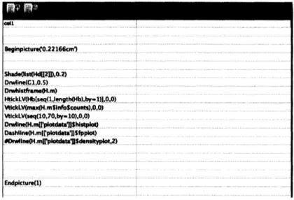
Users can easily finely-tune the existing graphical output according to his/her demands as

describedin section 3. Thiscanbedone byeitherofthe following twoways. The first is to type

the necessary commands in $R$ data editor (Figure 7), the other is by adding the commands to

the existing program using $R$’s edit commands. For example, ifwe want to shade the second

bar from the left, we simply need touse the following process dependent on the user interfaces:

graphical

_interface

case:

After typing fix(Cmd) _{in an open} $R$ consolewindow, an $R$data editor window appears

on

Figure 7 Window of$R$ data editor

command-line

_interface

case:

Add Insertcom$(^{\uparrow\dagger}$Cmd$|’,6,$ $|$

’Shade$($list(Hd$[[2]]$ ),$0.2)^{\dagger 1})$ to the existing program.After

adding other graphics and annotations to the plot, we obtain the graph illustrated below. It is

not necessary to delete other graphics and annotations in this example, however it is possible

to do so.

No. ofpersons

Histogram

23456 8 1012 15 20 25 30

Annual income

Figure 8 Finely-tuned graphic output for histogram

4.2

Program

for Boxplots

The program for creating boxplot output is as follows:

capnames $<-c(^{tI}$Sepal. Length”,”_{Sepal. Width“,}“_{Petal.Length“,}$1t$

Petal.Width$\mathfrak{l}1$

) Title $<-$ list$(^{1\dagger}Boxplot^{\mathfrak{l}\mathfrak{l}}$,“1”,$1|bf^{1I})$

Drwboxplot(iris[1; 4], $||BoxD$“_{, $c(10,10)$ , title$=Title$,} cap

$=Cap$,

ylab$=list(^{11\dagger 1})$ , ptsize$=5$, plot$=TRUE$)

$\#$ iris[1;4] is data set

Cmd $<$-BoxD$commands

fix(Cmd) $\#$ if necessary

Maketexfile(Cmd,$11f$ig.tex”)

The function Drwboxplot works on the same principle as the function Drwhistplot. We can

shade any box individually and indicate the figures in the $y$ axis showing the locations of

the boxes which stand for the median, and the 25th and 75th percentiles. After running the

program and adding other required graphics and annotations to the plot, we obtain the graph

below.

Boxplot

Sepal.Length Sepal.Width Petal.Length Petal.Width

Figure 9 Finely-tuned graphic output for boxplot

Boxplots arediagramsfor presentingnecessary information to see thecenter, spread, skew, and

length oftails in adata set. This type ofgraph allows us to compare many distributions in one

figure.

4.3

$K]\Gamma pic$

Metacommands

Cmdis amatrix whichis comprised of a number of character strings, as we saw in the previous

subsection. Each character string stands for a $I\mathfrak{g}r_{P}ic$ command as listed in the example in

section 4.1. When the draw function Drwhistplot or Drwboxplot is executed, Cmd is

substi-tuted for the relevant variable H.$m$ or $BoxD$, and the draw function interprets character strings

stored in Cmd as $Iqr_{P}ic$ commands and executes them. Maketexfile also interprets character

strings storedin Cmdas $Iqr_{P}ic$ commands and executes them. $R$ isequippedwith the function

eval (parse(text$=a||$ character string”) which parses a character stringand thenevaluates

it in the environment from which eval (parse$(\cdots)$) was called. Using this function allows the

draw functionsDrwhistplot and Drwboxplot, and Maketexfile to work as a single command

5

Conclusion

and

Further

Development

We havedeveloped an R-based $I\Phi r_{P}ic$ plug-in to yield high-quality statistical graph output to

be embedded into standard $BEX$. Currently the draw function is able to produce histograms

and boxplots. In the future we intelld to expand the scope of the function to enable the

output of a greater range of statistical graphs designed to help the learner better understand

statistical ideas. We will enhance the power of the R-based $I\Phi r_{P}ic$ plug-in, bringing increased

functionality, and creating a user-friendly system.

References

[1] Kiyoshi Kitahara, Takayuki Abe, Masataka Kaneko, Satoshi Yamashita and Setsuo

Takato,”Towards a More Effective Use of $3D$-Graphics in Mathematics Education

-Utilization of KETpic to Insert Figures into LaTeX Documents-,,_{,to appear in The}

In-ternational Journal for Technology in Mathematics Education, Vol. 17, Number 3, 2010.

[2] Koshikawa, H., Kaneko, M., Yamashita, S., Kitahara, K., Takato, S.,: Handier Use of Scilab

to Draw Fine

_I4EX

Figures-Usage of$Iqr_{P}ic$Version forScilab-.Proc. ICCSA2010, IEEE

Press, 39-48

[3] M. Kaneko, T. Abe, M. Sekiguchi, Y. Tadokoro, K. Fukazawa, S. Yamashitaand S. Takato,

“CAS-aided Visualization in La TeX documents

_for

Mathematical Education,” Teaching

Mathematics and Computer Science, vol. 8, issue 1, (2010)

[4] A. Galvez, A. Iglesias and S. Takato, “New Matlab-Based KETpic Plug-In

_for

High-Quality

Drawing

_of

Curves,” 2009 International Conference on Computational Sciences and its

Ap-plications, IEEE Press, 2009, pp.123-131.

[5] M. Sekiguchi, M. Kaneko, Y. Tadokoro, S. Yamashita and S. Takato, A New Application

of

CAS to La TeX-Plottings,” Lecture Notes in Computer Science, Springer-Verlag, 4488,

pp. 178-185, 2007.

[6] M. Sekiguchi, S. Yamashita and S. Takato, “Development

_of

a Maple Macro Package

Suit-able

_for

Dmwing Fine TeX-Pictures,” Lecture Notesin Computer Science, Springer-Verlag,

4151, pp. 24-34,

2006.