Numerical Solution Of Partial Integro-Differential Equation Using Legendre Multi Wavelets

(1)

西南交通大学学报

第 55 卷第 2 期

2020 年 4 月

JOURNAL OF SOUTHWEST JIAOTONG UNIVERSITY

Vol. 55 No. 2

Apr. 2020

ISSN: 0258-2724 DOI：10.35741/issn.0258-2724.55.2.24

Research article Mathematics

N

UMERICAL

S

OLUTION

O

F

P

ARTIAL

I

NTEGRO

-D

IFFERENTIAL

E

QUATION

U

SING

L

EGENDRE

M

ULTI

W

AVELETS

使用传奇多小波的局部积分-微分方程数值解

Amina Kassim Hussain

Department of Material Engineering, College of Engineering, Mustansiriyah University Baghdad, Iraq

[email protected], [email protected]

Received: August 18, 2019 ▪ Review: October 15, 2019 ▪ Accepted: February 27, 2020 This article is an open access article distributed under the terms and conditions of the Creative Commons Attribution License

(http://creativecommons.org/licenses/by/4.0)

Abstract

It is very important to state the initial assumptions for the description of physical phenomenon in the case of partial integro-differential equation. The parabolic equations and boundary conditions can be used to define the time-dependent diffusion process. The integro-differential equation is the combination of integration and derivatives. It is part of the technology, which includes science and engineering. Various models that cover the area of science and engineering are available. Moreover, variable techniques are accessible to solve the integro-differential equations. Numerical method is an important way to solve the challenges in the field of science and industry. To improve efficiency, the companies were working on computer simulation. For reliability, flexibility, and inexpensiveness, the numerical methods are preferred. Linear Legendre multi wavelets form a collocated method based on the numerical solution of one-dimensional parabolic partial integro-differential equation of diffusion type. In this study, we aim to study the diffusion method of numerical solution for the integro-partial differential equation. The diffusion method, its basic concept, and other methods used to solve integro-partial differential equations are also studied in detail. The proposed numerical method is useful to different benchmark problems and provides efficient, accurate, and robust results.

Keywords: Numerical Method, Partial Differential Equation, Partial Integro-Differential Equation, Partial Integro-Differential Equation of Diffusion Type

摘要

在部分积分-微分方程的情况下，陈述描述物理现象的初始假设非常重要。抛物线方程和边界条件可用于定义时间相关的扩散过程。积分微分方程是积分和导数的组合。它是技术的一部分，包括科学和工程。提供涵盖科学和工程领域的各种模型。此外，可以使用可变技术来求解积分微分方程。数值方

(2)

法是解决科学和工业领域挑战的重要途径。为了提高效率，这些公司正在研究计算机仿真。为了可靠性，灵活性和便宜性，数值方法是优选的。线性勒让德多小波基于一维抛物型一维抛物型积分微分方程的数值解，形成了一种并置方法。在这项研究中，我们旨在研究积分偏微分方程数值解的扩散方法。还详细研究了扩散方法，其基本概念以及用于求解积分偏微分方程的其他方法。所提出的数值方法可用于解决不同的基准问题，并提供有效，准确和可靠的结果。 关键词: 扩散型数值方法，偏微分方程，偏积分微分方程，偏积分微分方程

I. I

NTRODUCTION

Recently various mathematical models such as stochastic equations, ordinary, partial, linear, nonlinear, fractional, integral, integro-differential equations are leads to functional equations. They have wide applications in various sectors such as physics, geology, chemistry, dynamic systems, industries, and so on.

The key point regarding the simulation process is the formation of the correct mathematical model. This model should be convenient for the physical phenomenon under research. A partial diﬀerential equation plays an important role in modeling various processes. The classical type PDEs models do not regenerate the relevant model. Partial diﬀerential equations fail when it comes to evaluate the classical PDE. Hence, the partial integro-differential equation comes into the picture. In recent years, many of the PIDEs-based models made, are superior to the classical model. This can be proven theoretically as well as practically [1].

Different types of solution topics and methods are available. Here we list a few of the solution topics like integral solutions, numerical integrations, dirac delta function, asymptotic, exponential stability, etc., as the solutions to various problems are acquired by a variety of different methods such as Diffusion type, Euler method, finite differentiation method, integral transform, integrating factor, crank nicolson, runge-kutta, finite element, finite volume, Galerkin, perturbation theory [2] and [3].

There are lots of problems which lack standard solutions like, partial integro-differential equations. Typically it is hard to solve partial integro-differential equations. Hence this leads to a birth of solutions with numerical approximations. PIDEs have different factors like nonlinearity non-local phenomena and multi-dimensionality, physical constraints and a higher number of variables. Hence, it is a huge challenge to solve such types of problem numerically as well as analytically. As we know, mathematical biology, fluid dynamics,

viscoelasticity, engineering, financial mathematics, and many other areas are facing problems involving partial integro-differential equations [4].

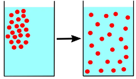
Basically, diffusion is the process of the transportation of molecules or species caused due to movement. Its dictionary meaning is to 'spread out'. There are various equations for diffusion. Here in this paper, we discuss the mathematical equation of diffusion type.

Figure 1. Diffusion process

The term 'diffusion' is given to the process which deals with the physics. With the help of examples, the term is described in Figure 1. We take one glass of water. A few particles are mixed in that water. Initially, all of the particles are located at the top of glass. After some time there is the random movement of particles known as 'diffusion' in water. The concept gradient is defined as the rate of change of the value of the quantity e.g. temperature, pressure, etc. The diffusion is dependent on the random movements of the particles. This results in mixing. We also say that mass transportation is in the absence of bulk motion. In the next section we also describe the term 'convection' with regards to diffusion.

II. B

ASIC

C

ONCEPT

This section consists of short introductions to various basic concepts. It includes numerical methods, partial differential equations, partial integro-differential equations (PIDE) and diﬀusion.

(3)

3

A. Numerical Methods

Basically, numerical analysis is a mathematical tool. It is designed to solve numerical problems. Solving numerical problems with a mathematical tool is known as a 'numerical method'. Stepwise flow with programming language is used to design the mathematical model known as the 'numerical algorithm'. There are various numerical methods available for solving numerical problems such as the iterative method, Newton–Raphson division, Newton's method, Horner's method rate of convergence, Taylor series method, runge-kutta methods, laplace transform method, elzaki transform, double elzaki transform linear, multistep methods and gear methods. Available numerical methods are used to solve real-world problems, i.e., dynamic systems. In cases of real-time systems, the initial conditions must be assumed before solving the problem [5].

B. Partial Differential Equations

Partial differential equations (PDEs) are classified as hyperbolic, parabolic, or elliptic.

The procedures used to solve these equations are different.

(1) Equation 1 is the example of Laplace’s equation, which comes under the heading of elliptic PDEs.

Similarly,

(2) (3) Equations 2 and 3 are examples of the wave equation and diffusion equation, which comes under the headings of hyperbolic and parabolic PDEs, respectively. These equations may be of the mixed type, which depend on the parameters’ values. Let’s consider the equation

(4) Equation 4 is known as Tricomi’s equation. Its conditions for PDE are y < 0 (hyperbolic), y = 0 (parabolic), and y > 0 (elliptic) [6].

C. Partial Integro-Differential Equations (PIDEs)

If we take the derivative of one variable with respect to another variable for variables that are related to each other, then this type of integro-differential equation (IDE) is known as ordinary. Generally, IDEs occur in the fields of mathematical physics and geology with respect to different variables. Then, these types of equations

are known as partial IDEs (PIDEs). Any functional equations that consist of unknown functions are identified as an IDE with differential and integral operations on a given function. There are various types of IDEs available; a few are listed here, such as linear ordinary and nonlinear IDEs [7].

D. Diffusion

Diffusion concept is based on with Fick's laws of diffusion. Their mathematical results are generating from random walk diffused particles. As per Fick's laws, diffusion fluxes are proportional to negative gradient.

In the previous section in short, we discuss the diffusion concept. Here we focus deeply. The equation with convection–diffusion comes under the partial differential equation with parabolic parameters. It describes the physical environment, i.e., the phenomenon where the transformation of energy inside a physical system has occurred due to convection and diffusion processes.

(5) Here, x belongs to , which is equal to [0, 1] and t belongs to J, which is equal to [0, T]. The ‘x’ has initial and boundary conditions, as follows:

where m ≥ 0 is the constant of the convection process, and b > 0 is the constant of the diffusion process.

Equation 5 indicates convection–diffusion in the form of an integral term, which is equal to 0. It is necessary to analyze the heat transfer model or system where a high temperature allows them to pass through the porous medium. It shows the effective conversion of gas enthalpy to thermal radiation in a porous medium [8].

III. M

ATHEMATICAL

C

ONCEPTS

Before moving forward, we will discuss some mathematical numerical methods that are used to solve differential equations. A few methods are briefly listed here, including the decomposition method, the Adomian decomposition method (ADM), the finite difference method (FDM) and the product trapezoidal method and the weakly singular kernel method. Each method is brifly explained below.

(4)

Various methods are available to perform decomposition of the mean. In this method, the main program is divided into subprograms. There are various types of decomposition methods available, such as the adomain decomposition method (ADM), the domain decomposition method, etc. [9].

B. Adomian Decomposition Method (ADM)

The ADM was invented in 1980 to solve real-world problems associated with semi-analytical methods. Many studies have been carried out using the ADM, which includes a linear–non-linear equation, PDE, integral equation, integro-differential equation, homogeneous, and non-homogeneous equation. The important issue for ADM is the Adomian polynomial employment, which facilitates the solution of convergence for the nonlinear part of the equation.

C. Finite Difference Method (FDM)

This method is based on the differential equation. To solve problems, the matrix algebra technique is used. This method is very useful for solving differential equations [10].

D. Product Trapezoidal Method

In this type of numerical analysis, the trapezoidal rule is used to approximate the definite integral [13]. This rule works by approximating the region or coverage under a graph having the function f(x).

E. Weakly Singular Kernel Method

Weakly-singular kernels appear frequently in the boundary integral equation method for solving elliptic equations. With weakly singular kernels k(x, y); the right- hand side f can be smooth or have irregularities.

F. One-Dimensional Diffusion Equation

Here, we consider the diffusion equation, which is one-dimensional. This equation is time dependent.

0 < x < 1, 0 < t < T (6)

Put through the initial condition u(x, 0) = f (x), 0 < x < 1, the boundary condition is u(1, t) = g(t), 0 < t ≤ T.

The non-local boundary conditions are shown in the following equation (7).

where 0 < t ≤ T and 0 < b < 1.

In this case f, g, b, s, and m are known, and we want to determine function u. This is basically a one-dimensional parabolic equation. This equation includes the parabolic equation with the nonlocal conditions mentioned above. The nonlocal conditions differ from classical conditions. The concept of the nonlocal problem is important in cases of transport of passive and reactive model in the field of research mathematics in the presence of an aquifer. Parabolic problems arise from thermo-elasticity [11].

G. Proposed Method for the PIDE of Diffusion Types

Linear Legendre multi-wavelets, which are collocation method-based, are used as the numerical solution of the one-dimensional parabolic PIDE of diffusion types. The proposed numerical method is useful for different benchmark problems. The proposed method provides results with efficiency, accuracy, and robustness.

Here, we consider the equation:

assuming the initial condition and the conditions of the Dirichlet boundary, as follows:

Here,

are the boundary conditions.

Another assumption is that function h (x,t) and k (x, t) are smooth.

Analytical solutions are unavailable for PIDEs, so one way of reaching a solution is by finding approximate solutions. There are many methods that have been introduced to reach a solution, such as the curve length method, the Tau method, the Sobolev gradient method, the explicit iterative method, the flatness method, the homotopy analysis transform method, the operational matrix method, and the collocation method. We use the concept of wavelets in the theory of approximation. This concept is useful in cases of numerical solutions for fractional diffusion wave equations, partial differential equations, ordinary differential equations, and integro-differential equations. A proposed

(5)

5

method uses different types of wavelets such as Battle-Lemarie wavelets, Haar wavelets, and Daubechies wavelets.

H. Linear Legendre Multiwavelets

A mother wavelet is generated from the dilation as well as the translation of a unit, i.e., a single function. Due to variations in parameter a, b is the continuous form of wavelets obtained, which is described below.

If a and b are restricted to discrete values, then . Now we get:

The mother wavelet fulfills the condition w(x) = 0. Here, we consider a discrete wavelet family.

I. Numerical Procedure: One-Dimensional Partial Integro-Differential Equation

We used linear Legendre multiwavelets to obtain solutions of one-dimensional as well as two-dimensional PIDEs. We use the one-dimensional equation below.

where the initial condition is:

We use the collocation method with linear Legendre multiwavelets. Here, we assume the collocation method for one-dimensional. We will now discuss this method with the help of some test examples [12].

Example 1: Now, consider the diffusion

problem:

where x belongs to Ω and t belongs to [0,1]. Then, the initial conditions are:

Here, we get the exact solution for the above problem as:

The h(t) for this problem is:

The exact solution of the above problem includes a hyperbolic function. The same problem is tested with two-dimensional linear Legendre multiwavelets. Table 1 shows the maximum absolute errors at different times.

Table 1.

Max absolute errors at different time (example 1)

t N=4 ×4 N=8×8 N=16×16 N=32×32 0.1 1.40×10-4 1.81×10-6 9.21×10-7 9.52×10-8 0.2 5.58×10-5 1.35×10-5 2.33×10-6 1.55×10-6 0.3 1.81×10-4 7.30×10-5 1.99×10-6 1.09×10-6 0.4 1.58×10-4 4.40×10-5 1.78×10-5 1.26×10-6 0.5 1.81×10-3 3.77×10-4 7.74×10-5 1.73×10-5 0.6 5.82×10-4 4.52×10-5 9.52×10-6 3.80×10-6 0.7 2.15×10-4 _2.37×10-5 _2.02×10-5 _4.66×10-6 0.8 4.26×10-4 8.33×10-5 2.32×10-5 3.47×10-6 0.9 1.06×10-4 1.08×10-4 1.20×10-5 7.18×10-6 1.0 1.02×10-3 3.43×10-4 8.64×10-5 2.03×10-5

Example 2: Now, we consider the diffusion

problem.

Here,

For this problem, we apply two-dimensional linear Legendre multiwavelets, and we obtain the results in Table 2 and Figure 2. From Table 2 we can easily understand the absolute error.

Table 2.

Max absolute errors at different time (example 2)

t N=4×4 N=8×8 N=16×16 N=32×32 0.0625 1.03×10-3 7.44×10-5 4.63×10-6 1.22×10−5 0.1875 1.90×10-4 7.56×10-5 1.23×10-5 2.47×10−5 0.3125 7.08×10-4 1.46×10-4 2.57×10-5 3.58×10−5 0.4375 1.51×10-4 7.59×10-5 4.22×10-5 4.56×10−5 0.5625 2.62×10-3 1.22×10-4 6.07×10-5 5.39×10−5 0.6875 7.24×10-4 _1.06×10-4 _8.19×10-5 _6.05×10−5 0.8125 1.56×10-3 4.72×10-5 1.07×10-4 6.49×10−5 0.9375 4.30×10-4 2.19×10-4 1.38×10-4 6.64×10−5

(6)

Exact solution Approximate solution Figure 2. Graph of exact and approximate solution

IV. C

ONCLUSION

In this paper, we studied the numerical method for solving diffusion-type equations. With the help of some examples, we discussed the collocation method. If we are going to increase number of collocation points, the maximum absolute errors continue to decrease. The maximum absolute error is time independent. Here, we observe the oscillating behavior with a fixed number of collocation points. Figure 2 also shows the same results for N = 32 * 32 for an exact as well as an approximate solution.

R

EFERENCES

[1]

PINTO, L.M.D. (2013) Parabolic

Partial

Integro-Differential

Equations:

Superconvergence

Estimates

and

Applications. Doctoral thesis, University of

Coimbra.

[2]

BIAZAR, J. and ASADI, M.A.

(2015)

FD-RBF

for

partial

integro-differential equations with a weakly singular

kernel.

Applied

and

Computational

Mathematics, 4 (6), pp. 445-451.

[3]

YOON,

J.M.,

XIE,

S.,

and

HRYNKIV, V. (2012) Two numerical

algorithms for solving a partial

integro-differential equation with a weakly singular

kernel.

Applications

and

Applied

Mathematics, 7 (1), pp. 133-141.

[4]

SALMAN, Z.A.N. (2006) Partial

integro-differential equations: classification

&

solutions.

Available

from

https://kipdf.com/partial-integro-differential-

equations-classification-solutions_5ab21e751723dd349c810e76.html

.

[5]

KURTH, P. (2014) On a New Class

of Partial Integro-Differential Equations.

Journal

of

Integral

Equations

and

Applications, 26 (4), pp. 497-526.

[6]

DAGMAR, I. (2017) Numerical

solution of Reaction-Diffusion Problems.

Basel:

Computational

Biology

Group,

Department for Biosystems Science and

Engineering, ETH Zurich, Swiss Institute of

Bioinformatics.

[7]

NIGATIE, Y. (2018) The finite

difference methods for parabolic partial

differential equations. Journal of Applied and

Computational Mathematics, 7 (3), pp. 1-4.

[8]

FAHIM, A. and ARAGHI, M.A.F.

(2018) Numerical solution of

convection-diffusion equations with memory term based

on sinc method. Computational Methods for

Differential Equations, 6 (3), pp. 380-395.

[9]

FORTIN, N., LEMIEUX, T., and

FIRPO, S. (2010) Decomposition Methods in

Economics. Cambridge: National Bureau of

Economic Research.

[10]

CAUSON, D.M. and MINGHAM,

C.G. (2010) Introductory Finite Difference

Methods for PDEs. London: Bookboon.

[11]

DEHGHAN, M. (2003) On the

Numerical

Solution

of

the

Diffusion

Equation

with

a

Nonlocal

Boundary

Condition.

Mathematical

Problems

in

Engineering, 2, pp. 81-92.

[12]

AZIZ, I. and KHAN, I. (2017)