Successive homoclinic doublings bifurcations from oribt-flip

Successive

homoclinic doublings

bifurcations

from

orbit-flip

Motomasa

Komuro

(小室元政)

Department

of Mathematics

The

Nishi-Tokyo University

2525

Yatsusawa,

Uenohara-mati

Yamanashi 409-01, Japan

Collaboration with

Hiroshi

Kokubu

Department

of Mathematics

Faculty of

Science

Kyoto University

Kyoto

606-01,

Japan

[email protected]

and

Hiroe

Oka

Department

of Applied Mathematics and Informatics

Faculty of

Science

and Technology

Ryukoku

University

Seta,

Otsu 520-21,

Japan

[email protected]

1

Introduction

Motivation

Extensivestudyhasrecently been madeforbifurcations occurring

in aneighborhoodof a codimensiontwo homoclinicorbit in a three-dimensional

vector field, and in particular, it became known that some types of codimension two homoclinicorbits which are$\mathrm{b}\mathrm{i}$-asymptotic to hyperbolic equilibria with real principal eigenvalues can give rise to multiple homoclinic orbits; an N-times roundinghomoclinicorbit arises under perturbation in a tubular neighborhood

of the unperturbed orbit where $N$ being an integer ([27], [1], [11, 12], [25], [7]). Such a homoclinic orbit is referred to as an $N$-homoclinic orbit with respect to theoriginal unperturbedone. Thebifurcation of suchmultiplehomoclinicorbits

are, however, still far from being understood. For instance, when one varies the

eigenvalues of the equilibria it has been observed by a numerical simulation a very complicated bifurcation involving many such multiple homoclinic orbits.

See, for instance, Figure 4.1 and [10].

The purpose of this and forthcoming papers is to obtain a better under-standing of such complicated bifurcations for multiple homoclinic orbits by combining results from homoclinic bifurcation analyses with those from

nu-merical experiments. To be more precise, we shall take one particular type of codimension twohomoclinic orbits with realeigenvaluesin $\mathrm{I}\mathrm{R}^{3}$, called orbit-fiip, and study its bifurcation of multiple homoclinic orbits appearing in a tubular neighborhood of the original orbit-flip. The main interest of the present pa-per lies in the

occurrence

of successive homoclinic doubling bifurcations under

an appropriate condition, which is a part of the total bifurcations for multiple homoclinic orbits. Here the homoclinic doubling bifurcation refers to the bifur-cation of a homoclinic orbit changing into a twice rounding homoclinic orbit in a tubular neighborhood of the original one. The homoclinic doubling bifurca-tion associated to real principal eigenvalues was first studied by $\mathrm{Y}\mathrm{a}\mathrm{n}\mathrm{a}\mathrm{g}\mathrm{i}\mathrm{d}\mathrm{a}[27]$

where he asserted that there are three kinds of codimension two homoclinic orbits that can undergo the homoclinic doubling bifurcations: these are now called (i) a homoclinic orbit with resonances, (ii) that of inclination-flip type,

and (iii) that of orbit-flip type. See [1], $[11, 12]$ and [25] for efforts toward

justi-fying and generalizing Yanagida’s original ideas concerning these three types of homoclinic doubling bifurcations. In this paper, we shall show the existence of

cascade of homoclinic bifurcations starting from a homoclinic orbit of orbit-flip type followed by those of inclination-flip type. Relation between such a global bifurcation and a local bifurcation from orbit-flip will also be discussed in the last section.

Continuous piecewise-linear vector fields Sincethe cascade of homoclinic doublings is a totally global bifurcation, we need an aid of numerical experi-ments in which we must choose a concrete set of ordinary differential equations that exhibits the desired bifurcation. In this paper we employ a family of con-tinuous piecewise-linear vector

_fields

for such a model equation. The advantage

of using such continuous piecewise-linear vector fields is that, firstly it is eas-ier to analyze dynamics and bifurcations of the vector fields because of their piecewise-linearity, and secondly, according to a general theory established by the second author of this paper ([14]), we can obtain a kind of normal forms for generic continuous piecewise-linear vector fields if one specifies the number ofregions on which the vector field is linear, and the normal form is completely characterized in the sense of linear conjugacy in terms of the eigenvalues at equilibria in each of these linear regions. This means that these eigenvalues are considered to be the bifurcation parameters of the normal form equations, which is suitablefor our purpose of this and subsequent papers. In our case, we use the normal form of piecewise-linear vector fields with two linear regions in

$1\mathrm{R}^{3}$, and hence it possesses six parameters in total. Moreover it is easy to derive

an explicit condition in terms of the eigenvalue parameters for theexistence of orbit-flip homoclinic orbits. Using this information, we can set up the model problem in a tractable way and perform very precise numerical experiments based on explicitly computed analytic formulas. The results obtained by such analyses and experiments will also be valid for general smooth vector fields, be-cause the homoclinic bifurcation theory only uses information from the return map along the original homoclinic orbit and hence the piecewise-linearity does

not lose essential information for it is constructed in the same way as in the smooth case.

Main results Using such a family of continuous piecewise-linear vector fields, we shall demonstrate the presence of the following global bifurcations in this paper: Since the original homoclinic orbit is assumed to be of orbit-flip type, it undergoes the first homoclinic doubling bifurcation and gives rise to a

2-homoclinic orbit. It then turns to be a homoclinic orbit of inclination-flip type after a slight change of parameters and thus undergoes the second doubling bi-furcation creating a 4-homoclinic orbit. This 4-homoclinic orbit becomes again

that of inclination-flip type for a further variation of parameters and we find

8-homoclinic orbit through the third homoclinic doubling bifurcation. By nu-merical experiments for our family of continuous piecewise-linear vector fields we can similarly see that each $2^{k}$-homoclinic orbit becomes that of inclination-flip

type and gives rise to a $2^{k+1}$-homoclinic orbit through the homoclinic doubling bifurcation. In fact we have observed up to $2^{6}=64$-homoclinic orbits through

these doubling bifurcations. Such precise numerical experiments could only be done by using piecewise-linear vector fields, since it is in general hard to find a homoclinic orbit as an intersection of the stable and unstable manifolds, but

for piecewise-linear vector fields, those manifolds are locally given by a straight

line or a plane and hence it is quite easy to find a parameter value where an

orbit precisely lies on these manifolds.

In order to explain this bifurcation more theoretically, we derive a two-parameter family of unimodal maps as singular limit of thePoincar\’emapsalong

homoclinicorbits. Welocate bifurcationcurves for this family of unimodal maps in the two-dimensional parameter space and these curves basically agree with thosefor the piecewise-linear vector fields. In particular, we show, using a stan-dard technique from the theory ofunimodal maps (see e.g. [2], [18], [19]), that there exists an infinite cascade of doubling bifurcations which corresponds to the sequence of homoclinic doubling bifurcations for the piecewise-linear vector fields describedabove. Since our unimodal map has a singularityat a boundary point of its domain of definition, the doubling bifurcation is slightly different

from that for standard quadratic unimodal maps, for instance the Feigenbaum constant associated to accumulation of the doubling bifurcations is different

from the standard value 4.6692.... Basic qualitative similarity between the bi-furcations of our unimodal map family and the piecewise-linear vector fields strongly suggest that there does also exist a cascade of homoclinic doubling bifurcations in our family of continuous piecewise-linear vector fields in a way described by their singular limit unimodal maps.

Acknowledgement. We are grateful to T. Matsumoto, K. Iori, Y. Kurimoto for stimulating discussions.

2

Preliminaries

Consider a family of vector fields $X_{\eta}$ on $1\mathrm{R}^{3}$ with a hyperbolic equilibrium

point $O$ and suppose that it admits a homoclinic orbit $\Gamma$ to the equilibrium

point for $\eta=0$ where the linearization matrix possesses eigenvalues $\lambda_{u}$ and

$-\lambda_{ss},$ $-\lambda_{s}$ with _{$-\lambda_{ss}<-\lambda_{s}<0<\lambda_{u}$}

.

The eigenvalues $\lambda_{u}$ and $-\lambda_{s}$ are

called principal. Then for sufficiently small $\eta,$ $X_{\eta}$ may possess a homoclinic

orbit rounding twice in a small tubular neighborhood of the original homoclinic

orbit. Such a bifurcation is referred to as homoclinic doubling

_bifurcation

and the bifurcating homoclinic orbit is called a doubled homoclinic orbit or a

2-homoclinic orbit with respect to the original one which is called the primary or 1-homoclinic orbit.

For the homoclinic orbit, we can generically expect the following two con-ditions to be satisfied:

(Ev) $\lambda_{u}\neq\lambda_{s}$;

(Asy) $\Gamma$ is tangent at $O$ to the eigendirection associated to $-\lambda_{s}$ as $t$ tends to $+\infty$

.

Besides the stable manifold denoted by $W^{s}(O)$

,

we can consider another invari-ant manifold which is tangent to the eigendirections associated with $\lambda_{u}$ and

$-\lambda_{S}$

.

In this paper we call it an extended unstable

manifold

which we denote by $W^{\mathrm{e}u}(O)$

.

Notice that the homoclinic orbit $\Gamma$ is contained in $W^{eu}(O)\cap W^{s}(O)$

.

Generically we have

(Tr) $W^{\mathrm{e}u}(O)$ and $W^{s}(O)$ intersect transversely along $\Gamma$

.

A degenerate homoclinic orbit arises by breaking one of these genericity

conditions, as in the following way.

Definition 2.1. Let $\Gamma$ be a homoclinic orbit of the vector field $X=X_{0}$

.

(Inc) $\Gamma$ is called a homoclinic orbit

of

inclination-fiip type, if (Ev) and (Asy)

hold,but (Tr) does not, namely, $W^{s}(O)$ and $W^{\mathrm{e}u}(O)$ are tangent along $\Gamma$;

(Orb) $\Gamma$ is called a homoclinic orbit

of

orbit-fiip type, if (Tr) and (Ev) hold, but

(Asy) does not, namely, $\Gamma$ lies in the strong stable manifold _$W^{ss}(O)$;

$({\rm Res})\Gamma$ is called a homoclinic orbit with resonance, if (Tr) and (Asy) hold, but

(Ev) does not, namely, the resonance condition $\lambda_{u}=\lambda_{s}$ is satisfied.

Remark 2.2. The proof of the center manifold theorem works as well for the existence of the extended unstable manifold $W^{eu}(O)$. See [8] for the proof. This

invariant manifold is not unique, but has the unique tangent space along the homoclinic orbit, and hence the condition (Inc), which is sometimes referred to as the strong inclination property ([3]), is independent of the choice of the extended unstable manifold.

Bifurcations to doubled homoclinic orbits were first studied in [5] in the case of the Shil’nikov-type homoclinic orbit, together with the non-existence of the homoclinic doubling bifurcation for homoclinic orbits with real principal eigenvalues under the generic conditions (Asy), (Tr) and (Ev). Yanagida [27] then claimed that there are the above three possibilities of more degenerate homoclinic orbits with real principal eigenvalues that can generate a doubled

homoclinic orbit under perturbation. Since [27], a lot of work has been carried out toward completing and generalizing Yanagida’s original ideas.

It was shown in [1] that the period-doubling bifurcation or the saddle-node

bifurcation for a periodic orbit occurs in a generic two-parameter unfolding of a homoclinic orbit with resonant eigenvalues, depending whether the homo-clinic orbit is twisted or non-twisted. Similar bifurcations are also shown for inclination-flip homoclinic orbits ([11, 12]) with the ratio $\nu=\frac{}{\lambda}\lambda\perp_{u}$ of the

princi-pal eigenvalues $\mathrm{s}\mathrm{a}\mathrm{t}\mathrm{i}_{\mathrm{S}}\mathrm{f}\mathrm{y}\mathrm{i}\mathrm{n}\mathrm{g}\frac{1}{2}<\nu<1$

.

Onthe other hand, if the ratio $\nu$ is smaller

than $\frac{1}{2}$, more complicated dynamics such as the shift dynamics accompanied

by rich bifurcation phenomena in their creation possibly appear ([4], [7]). In particular, Homburg, Kokubu and Krupa [7] proved the existence of suspension of the Smale’s horseshoe in unfoldings of an inclination-flip homoclinic orbit with $\nu<\frac{1}{2},2\nu<\mu=\frac{\lambda}{\lambda}\mathrm{A}\mathrm{a}u$ and described how $N$-homoclinic orbits are

cre-ated and destroyed in the unfolding. Sandstede [26] showed the existence of a shift dynamics in the unfolding of an inclination-flip homoclinic orbit with

$\mu<1,$ $\mu<2\nu$ using Lin’s methods [16]. Recently, the existence of H\’enon-like

strange attractors was proved in [22], using a result of Mora and Viana [20], in the case where $1<\mu+\nu,$ $\nu<\frac{1}{2},$ $\mu>K\nu$ with some large enough $K$

.

See also

[21] and [13] for relevant results.

With regards to the orbit-flip homoclinic orbits, Sandstede [25] has proven that homoclinic doubling and homoclinic $N$-tupling bifurcations _{$(N\geq 3)$} as well as the shift dynamics do occur in its unfolding. There is also a numerical simulation done by [10] for piecewise-linear vector fields involving an orbit-flip

homoclinic orbit which shows interesting bifurcation curves for N-homoclinic

orbits with $2\leq N\leq 11$. Our work was inspired by this last result.

Here we state a theorem concerning the homoclinic doubling bifurcations

for homoclinic orbits of inclination-flip or orbit-flip type. Consider thefamily of vector fields $X_{\eta}$ with a hyperbolic equilibrium point $O$

.

This theorem

summa-rizes some results from [12] and [25].

Theorem 2.3. Let$X_{\eta}$ be a generic two-parameter family

of

vector

fields

which

has either an orbit-fiip or an inclination-fiip homoclinic orbit $\Gamma$ at

$\eta=0$

.

Then

the following holds:

(1)

_If

$1<\nu=arrow\lambda_{u^{f}}\lambda$ the homoclinic doubling

bifurcation

does not occur.

(2)

_If

$\frac{1}{2}<\nu<1$ and $\mu=\underline{\lambda}\lambda_{u}^{\Delta \mathrm{A}}>1$, the homoclinic doubling

bifurcation

occurs.

More precisely, there exists a local change

_of

parameters at $\eta=0$ $\epsilon=(\epsilon_{1},\mathcal{E}_{2})=\epsilon(\eta)$,

$\epsilon_{2}$ $=$ $\kappa_{2H}(\epsilon_{1})$ $(\epsilon_{1}\geq 0)$, $\epsilon_{2}$ $=$ $\kappa_{PD}(\mathcal{E}_{1})$ $(\epsilon_{1}\geq 0)$,

$\epsilon_{2}$ $=$ $\kappa_{SN}(\epsilon_{1})$ $(\epsilon_{1}\leq 0)$,

in the parameterspace such that a $p_{\dot{\mathcal{H}}m}ary$homoclinic orbit persists along

$\epsilon_{2}=0$ whereas a doubled homoclinic orbit

bifurcates

along _{$\epsilon_{2}=\kappa_{2H}(\epsilon_{1})$},

a $pe7\dot{\tau}odiC$ orbit undergoes the period doubling

bifurcation

along

$\epsilon_{2}=$ $\kappa_{PD}(\epsilon_{1})$, and the saddle-node

bifurcation

occurs

for

$pe\gamma\dot{\eta}odiCorbit_{\mathit{8}}$ along $\epsilon_{2}=\kappa_{SN}(\epsilon 1)$

.

Moreover,

$\kappa_{2H}(\epsilon_{1})$ $\approx\epsilon_{1}\frac{1}{1-\nu}$,

$\kappa_{PD}(\epsilon_{1})$ $\approx c\epsilon_{1}\frac{1}{1-\nu}$

for

some $0<c<1$,

$\kappa_{SN}(\epsilon_{1})$ $\approx$ $c’| \epsilon_{1}|\frac{1}{1-\nu}$

for

some $c’<0$.

See also [17] and references therein for more information.

Next we shall derive a two-parameter family of one-dimensional maps in

order to study the dynamics and bifurcations that occur in an unfolding of orbit-flip homoclinicorbits. This family is obtained bytaking the singular limit of the two-dimensional return maps along the homoclinic orbit as the strong

stable eigenvalue going$\mathrm{t}\mathrm{o}-\infty$.

Let $X_{\eta}$ bethe generic two-parameterunfolding as ab$o\mathrm{v}\mathrm{e}$ which possesses an

orbit-fliphomoclinicorbit $\Gamma$ to a hyperbolic equilibrium point _$O$

at $\eta=0$

.

$\Gamma$ lies

in theintersectionof the unstable andstrongstable manifolds $W^{u}(O)\cap W^{s}s(o)$

.

Wechoose the $(x, y, z)$-coordinatesin such a way that the _{localstable, unstable}

and strong stable manifolds are given by

$W_{l_{oC}}^{u}(O)=\{x=y=0\}$

,

$W_{l_{\mathit{0}}c}^{s}(o)=\{Z=0\}$, $W_{l\circ}^{ss}(\mathrm{C}O)=\mathrm{t}X=Z=0\}$ in a neighborhood of $O$

.

We assume for simplicity that the vector fields

$X_{\eta}$

are unifornly smoothly linearizablein a neighborhood of$O$ containing the unit cube $[$-1,$1]^{3}$, and take the two cross sections

$\Sigma^{0}=\{y=1\}$, $\Sigma^{1}=\{Z=1\}$

which are transverse to the homoclinic orbit F. Then the Poincar\’e map for $X_{\eta}$

along $\Gamma$ will be given by composition of the

the local map: $\Sigma^{0}arrow\Sigma^{1}$ ;

$\mapsto$

,

the global map: $\Sigma^{1}arrow\Sigma^{0}$ ; $-\rangle$

where $\mu$ – $\underline{\lambda}_{\mathrm{B}}\lambda_{u}$ and $\nu=\frac{\lambda}{\lambda}\mathrm{A}u$

.

Note that the constants, in particular, $p$ and $q$

may depend on the unfolding parameter $\eta$

.

Sincethe orbit-flip homoclinic orbit

exists when $(1, 0,0)$ is mapped to $(0,1,0)$ under the global map, we have

$p(\eta)=q(\eta)=0$

.

Therefore the parameter $\eta$ should be taken in such a way that

$\frac{\partial(p,q)}{\partial(\eta 1,\eta_{2})}|_{\eta=0}\neq 0$

.

In other words, $(p, q)$ can be thought of as unfolding parameters, and

conse-quently, the return map $h$ takes the form

$(x, z)\mapsto++$

.

Here we consider the case that the strongstable eigenvalue has a verylarge

modulus so that we can neglect the term involving $z^{\mu}$

.

Then themost dominant

terms in the return map reduce to give a one-dimensional map $z \mapsto\alpha(z-q+\frac{\gamma p}{\alpha})z^{\nu}+q$,

or, by rescaling the variable and parameters,

$f(x)=(x-a-b)x^{\nu}+b$

.

Notethat here we have assumed $\alpha>0$for simplicity, since the other casecanbe

treated similarly. In the next section we fix $\nu$ as being $\frac{1}{2}<\nu<1$ and consider

the bifurcation of this two-parameter family of one-dimensional maps that are

3 Analysis of reduced

one-dimensional maps

In this section we shall show that the two-parameter family of maps

$f(x;a, b)=(x-a-b)x^{\nu}+b$ $( \frac{1}{2}<\nu<1)$

possesses an infinite sequence of special doubling bifurcations that can be inter-preted as homoclinic doubling bifurcations of corresponding vector fields. First we note that the orbit of $0$ for the one-dimensional map corresponds to the

unstable manifoldof the equilibrium point for thevector field, and therefore we

only consider the maps on the interval $[0, f(\mathrm{o})]=[0, b]$ and trace the orbit of $0$

as long as it stays in this interval. This map is in generala unimodal map with a minimum which can be either positive or negative depending on the param-eters. In particular, the map with the parameters $(a, b)=(\mathrm{O}, 0)$ corresponds to the vector field with an orbit-flip. The curve which can be interpreted as the persistence curve for 1-homoclinic orbit coming out from theorbit-flip point is given by the condition that $0$ is a fixed point, namely _{$f(\mathrm{O})=b=0$}, whereas

the bifurcation curve for 2-homoclinic orbit is given by $f^{2}(0)=f(b)=0$, hence

$a=b^{1-\nu}$

.

These two bifurcation curves nicely fit with the bifurcation diagram for the vector fields that unfold an orbit-flip.

In general homoclinic orbits for vector fields correspond to periodic or-bits through $0$ for these one-dimensional maps, which is given by the equation

$f^{N}(0)=0$

.

Inclination-flip homoclinic orbits are interpreted as such periodic

orbits that pass through $0$ and the minimum point, and hence given by the

equations $f^{N}(0)=0,$ $f’(f^{N-1}(\mathrm{o}))=0$. In particular the inclination-flip

2-homoclinic orbit is given by the equations $f^{2}(0)=0$ and $f’(f(\mathrm{O}))=0$, or

equivalently, $(a, b)=(\nu^{\frac{1-\nu}{\nu}}, \nu^{\frac{1}{\nu}})$

.

It is hard to obtain explicit analytic

expres-sions for the $N$-homoclinic bifurcation curves with $N>2$, and hence, we use the following color diagram in order to visualize these curves.

We compute the number

$m= \min\{n\geq 1|f^{n}(0;a, b)\leq 0\}$

and assign a color code for each number $m$. Then we can draw bifurcation sets

with those assigned colors at each parameter value $(a, b)$. Figure $3.1(\mathrm{a})$ is one

example of such color diagrams. Each color code (except black) stands for a rounding number $m$, for instance, $m=1$ (blue), 2 (yellowish green), 3 (sky

blue), 4 (red), 5 (purple), 6 (yellow) and

7

(white). Higher rounding numbers

$m$ not larger than a number called Maxcount are coded as $(m-1)\mathrm{m}\mathrm{o}\mathrm{d} (7)+1$

.

If $m>\mathrm{M}\mathrm{a}\mathrm{x}\mathrm{c}\mathrm{o}\mathrm{u}\mathrm{n}\mathrm{t}$ or _$m=\infty$, then black is assigned. By definition, each point

Figure 3.1: Color-coded homoclinic bifurcation diagram for one-dimensional

map $f(x)=(x-a-b)x^{\nu}+b$ where $\nu=0.8$

.

(a) $(a, b)$-parameter space: $0.0\leq a\leq 2.0,0.0\leq b\leq 5.0$, Maxcount $=30$

.

(b) $(y_{*}, x_{*})$-parameter space: $0.0\geq y_{*}\geq-0.1,0.0\leq x_{*}\leq 2.0$, Maxcount $=30$

.

_(c) Successive homoclinic doubling bifurcations. Horizontal axis: $-9.5\leq\log_{1}\mathrm{o}y_{*}\leq 0.0$, Vertical axis:

$\log_{\mathrm{l}0^{b}0}\geq\log_{10}(b_{0}-x_{*})\geq-8.0$, where _{$b_{0}=1.151739$} and $\log_{\mathrm{l}0^{b}0}=0.061354$,

Maxcount $=1024$

.

number $m$, and hence it corresponds to a homoclinic bifurcation point for

m-homoclinic orbit. For example, the boundary $H_{4}$ of a red region with $m=4$

exhibits a 4-homoclinic bifurcation curve. In this way, it is quite easy to see the bifurcation curves for $N$-homoclinic orbits with various $N$

.

It can be seen that there is a curve at the envelop of all colored regions. This is given by the conditionthat the minimum value of $f$ is equal to $0$

,

since

if the minimum value is positive, then the orbit of $0$ never becomes negative

and hence, by the rule of color assignment, such a parameter value is colored

in black. This condition of the envelop is given by $f’(x_{*})=0,$ $f(x_{*})=0$, or

equivalently,

$a+b= \frac{1+\nu}{\nu}(\nu b)\frac{1}{1+\nu}$

.

Using this expression of the envelop, we make the change of parameters from

$(a, b)$ to

$x_{*}= \frac{\nu}{1+\nu}(a+b)$

,

$y_{*}=f(x_{*})=b- \frac{1}{\nu}(\frac{\nu}{1+\nu}(a+b))^{1+\nu}$

in such a way that the envelop is mapped to the $x_{*}$-axis. Figure3.1(b) exhibits

thecolor diagram with these new parameters, where we can more easily see the bifurcations, in particular several successive homoclinic doubling bifurcations.

This situation can be seen in more detail by taking $(\log x_{*}, \log y_{*})$ as new

pa-rameters. See Figure $3.1(\mathrm{c})$

.

Observe that the homoclinic doubling bifurcations

successively occur from 2-homoclinic orbit to $2^{10}=1024$-homoclinic orbit.

Since the homoclinic doubling bifurcation in vector fields corresponds to $0$

being a periodic orbit that passes through the minimum of the unimodal map$f$,

we shall rigorously show that there exists an infinitesequence of such successive

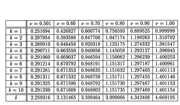
$\ovalbox{\tt\small REJECT}_{7}^{k}k--1k=k=k=2kk=4029k=k=k=9==50_{2}638027021020\mathrm{o}\mathrm{o}2899100\mathrm{o}^{2910_{300}^{110_{6}}}\mathrm{o}28790291325199919120_{311}128169375625140_{6}44001050606710606746467160802639369037682640_{5900_{9}^{94}}15321358575892094530500_{9}808477070092060949465941948484863080^{7}0_{8}^{318}8758779210^{4075}02156791010_{51}518115111111115150061145042515165711596323717735174175831753088952120121111129711122229291999219774332982636740_{514}^{7}774464239112271567185099951310^{99}140^{1}11401400_{15}^{2}404338900_{1}^{6}90_{961}151114970154147455\mathrm{s}192336$

Table 3.1: Successive homoclinic doublings and the Feigenbaum constant. For each valueof$\nu$, the parameter values $x_{*}$for inclination-flip $2^{k}$-homoclinic orbits

are shown, together with approximate values of the corresponding Feigenbaum constant $\delta$ computed fromthose data.

Theorem 3.1. The two-parameter family

_of

one-dimensional unimodal $map_{\mathit{8}}$ $f_{a,b}$ has a cascade

of

doubling

bifurcations

that can be interpreted $a\mathit{8}$ cascade

of

homoclinic doublings in the above $\mathit{8}ense$.

Proof.

We have only to consider the case where the minimum value of the

unimodal nap is $0$

.

This will reduce the two-parameter family of unimodal

maps to that with only one parameter:

$\tilde{f}_{b}=\{x-\frac{1+\nu}{\nu}(\nu b)\frac{1}{1+\nu}\}x+\nu b$,

since the condition that the minimum is equal to $0$ is given by

$y_{*}=b- \frac{1}{\nu}(\frac{\nu}{1+\nu}(a+b))1+\nu=^{0}$

.

The family $\tilde{f}_{b}$ is a $C^{1}$-family of unimodal maps that are continuous and onto

over theinterval $[0, b]$ and of$C^{1}$ on_{$(0, b]$}

.

Therefore this is almost what is called

the full family in the sense of Collet-Eckmann, for which the intermediate value theoremfor kneadingsequences holds. See [2], in particular Theorem III.1.1 for

the detail. We can apply this theorem to our family by modifying the proof of Theorem III.1.1 in [2], or more simply by looking at the second iterate $\tilde{f}_{b}^{l}$ as

follows: Since we assume the exponent $\nu$ satisfying $\frac{1}{2}<\nu<1$, it is easy to see

that $\tilde{f}_{b}^{2}$ restrictedto $[x_{0}, b]$ is exactly a full family of $C^{1}$-unimodalmaps without

any singularity, where $x_{0}$ standsfor the unique fixed point for

$\tilde{f}_{b}$

.

Since we have

computed the existence of thefirst doubling bifurcation point, we concludethat the cascade of doubling bifurcations occurringin $\tilde{f}_{b}^{2}$ gives the desired sequence.

We have numerically computed the Feigenbaum constants for the doubling bifurcations in the family $\tilde{f}_{b}$ with various exponent $\nu$

.

It should be noted that

when $\nu=1$

,

the Feigenbaum constant is close to the standard value 4.6692...,

but it is not, when $\frac{1}{2}<\nu<1$

.

Our data for the Feigenbaum constants resemble

to similar data for the unimodalmaps $x\vdasharrow 1-a|x|$( with $1<\zeta<12$ computed in [9] where the exponent (corresponds to $2\nu$ in our case.

4

Successive homoclinic

doublings

in

PL

vector fields

4.1 Normal forms of

three-dimensional two-region

proper piecewise-linear vector fields

We shall first summarize results for normal forms of three-dimensional proper two-region piecewise-linear vector fields. Since the proper condition which will be defined later is generic, they form an important class in the study of bifurca-tions for continuous piecewise-linear vector fields. In particular it can be shown that normal forms of proper systems are determined by elementary symmetric polynomial of eigenvalues in each linear region as described below.

Given a non-zero vector $\alpha\in 1\mathrm{R}^{3}$

,

define a plane

$V=\{_{X}\in \mathrm{R}^{3}|\langle\alpha,x)=1\}$

(where $\langle\cdot,$$\cdot\rangle$ denotes the usual inner product) and half spaces

$R_{\pm}=\{_{X\in]}\mathrm{R}3|\pm(\langle\alpha, x\rangle-1)>0\}$

.

Consider a vector field defined by an ordinary differential equation

$\frac{dx}{dt}=X(X)=\{$

$Ax$, $(x\in R_{-})$

(4.1) Bx-p, $(_{X\in}R_{+})$

,

where $A$ and $B$ are $3\cross 3$ matrices, and $p\in \mathrm{R}^{3}$ (all elements of $\mathrm{R}^{3}$ are column

vectors, unless otherwise stated). We call the vector field a three-dimensional two-region piecewise-linear vector field, and the plane $V$ the boundary of the

$B=A+p\alpha^{\tau}$

.

See [17, Lemma 2.5.1].

Definition 4.1. Two vector fields $X$ and $X’$ on $\mathrm{R}^{3}$ are linearly conjugate if

there is a non-singular matrix $H\in GL(3, \mathrm{R})$ such that

$HX(x)=X’(H_{X})$ for all $x\in 1\mathrm{R}^{3}$

.

Definition 4.2. A vector field $X$ defined by (4.1) is proper if any A-invariant proper linear subspace $E\subset \mathrm{R}^{3}$ intersects with the boundary $V$, i.e.,

$A(E)\subset E$ and $0<\dim(E)<3\Rightarrow E\cap V\neq\phi$

.

(4.2)

Theorem 4.3.

Any proper $Continuou\mathit{8}$ three-dimensional two-region piecewise-linear vector

field

given by

$X’(x)$ $=A’x+ \frac{1}{2}p’\{|\langle\alpha’, X\rangle-1|+((\alpha’, x\rangle-1)\}$

$=$ $\{$

$A’x$, $(\langle\alpha’, x\rangle-1\leq 0)$

$B’x-p’$, $(\langle\alpha’, X\rangle-1\geq 0)$,

$i_{\mathit{8}}$ linearly conjugate to the vector

field defined

by

$X(x)$ $=$ $Ax+ \frac{1}{2}p\{|\langle\alpha, x)-1|+(\langle\alpha, x\rangle-1)\}$,

$=$ $\{$

$Ax$, $(\langle\alpha, x)-1\leq 0)$

Bx-p, $(\langle\alpha, x\rangle-1\geq 0)$, whe re

$\alpha=(1,0,0)^{T}$, $p=(C_{1},c2, C3)^{\tau}$,

$A=$

,

$B==A+p\alpha^{\tau}$

$a_{1}=\lambda_{1}+\lambda_{2}+\lambda 3,$ $a_{2}=-(\lambda_{1}\lambda_{2}+\lambda 2\lambda 3+\lambda_{3}\lambda_{1}),$ $a_{3}=\lambda_{1}\lambda 2\lambda 3$,

$b_{1}=\nu_{1}+\nu_{2}+\nu_{3},$ $b_{2}=-(\nu_{1}\nu_{2}+\nu_{2}\nu 3+\nu 3\nu_{1}),$ $b_{3}=\nu_{1}\nu_{2}\nu_{3}$,

$\lambda_{1},$$\lambda_{2},$$\lambda_{3}$ being the $eigenvalue\mathit{8}$

of

$A$ and

$\nu_{1},$$\nu_{2},$$\nu_{3}$ being those

of

$B$

.

Moreover, when $\det(B)=b_{3}\neq 0$, we can write

$X(x)=\{$$Ax$, $(\langle\alpha,x\rangle-1\leq 0)$

$B(x-P)$, $(\langle\alpha, x\rangle-1\geq 0)$, where

$P=(1- \frac{a_{3}}{b_{3}},$$\frac{c_{1}a_{3}}{b_{3}},$$\frac{c_{2}a_{3}}{b_{3}})$

.

See [17, Subsection 2.5.1] for the proof of this theorem.

The vector field $X$ is determined by $\rho=(a_{1}, a_{2}, a_{3}, b_{1}, b_{2}, b_{3})\in \mathrm{R}^{6}$, which will be called the eigenvalue parameters. Define the boundary $V$ by

$V=\{_{X}\in \mathrm{R}^{3}|\langle\alpha, x\rangle=1\}$, and set

$V_{\pm}=\{x\in V|\pm\langle\alpha,Ax\rangle>0\}$

.

If $\lambda.\cdot(i=1,2,3)$ is real, then the vector $oC_{i}arrow$

gives an eigenvector of $A$ associated with $\lambda_{i}$, where

$C_{i}=(1, \lambda_{i}, \lambda_{i}^{2})T\in V$

.

(4.3)

Assume $\lambda_{1}$ and $\lambda_{2}$ are negative real and $\lambda_{3}$ is positive real, whereas

$\nu_{1}$ and $\nu_{2}$ are a pair of complex-conjugate numbers and $\nu_{3}$ is real. Denote

$\nu_{1},$$\nu_{2}=\sigma\pm\omega\sqrt{-1}$, $\nu_{3}=\gamma$

.

Since an eigenvector for $\lambda_{i}$ is given by (4.3), the one-dimensional

unsta-ble eigenspace $E^{u}(O)$ and the two-dimensional stable eigenspace $E^{s}(O)$ for

$O=(\mathrm{O},0,0)^{T}$ are given by

$E^{u}(O)=\{x\in 1\mathrm{R}^{3}|x=r(1, \lambda_{3}, \lambda_{3}^{2})^{T}, \langle\alpha, x\rangle-1\leq 0, r\in \mathrm{R}\}$,

$E^{s}(O)=\{x\in \mathrm{R}^{3}|\langle u,x\rangle=0, \langle\alpha,x)-1\leq 0\}$,

where $u=$ $(-1, \frac{\lambda+\lambda}{\lambda_{1}\lambda_{2}}, -\frac{1}{\lambda_{1}\lambda_{2}})$

.

The intersection $E^{s}(O)\cap V$ is thus given by

$E^{s}(O)\cap V=\{x=(x^{1},x^{2}, x^{3})\in 1\mathrm{R}^{3}|\langle u,x\rangle=0, x^{1}=1\}$

.

(4.4) If $\lambda_{2}<\lambda_{1}<0$, the strong stable eigenspace $E^{ss}(O)$ is given by

$E^{ss}(O)=\{x\in \mathrm{R}^{3}|x=r(1, \lambda_{2,2}\lambda^{2})^{T}, \langle\alpha, x\rangle-1\leq 0, r\in 1\mathrm{R}\}$

.

Take a point $C_{3}=(1, \lambda_{3,3}\lambda^{2})^{T}\in V_{+}$ on the local unstable manifold of $O$ and consider its entire orbit $\mathcal{O}(C_{3})$

.

The integer $m>0$ is called the rounding

number of the orbit if

Figure 4.1:

Color-coded

homoclinic bifurcation diagram for three-dimensional continuous piecewise-linear vector field with $\lambda_{1}=-0.2,$ $\lambda_{2}=-0.4,$$\lambda_{3}=$ $0.3,\omega=1.0$

.

$(\mathrm{a})$ Horizontal axis: $0.0\geq\gamma\geq-0.26$, Vertical axis: $0.0\leq\sigma\leq 0.3$,

Maxcount $=20$

.

(b) Enlargement of (a). Horizontal axis: $0.0\geq\gamma\geq-0.26$,

Vertical axis: $0.1\geq H_{1}(\gamma)-\sigma\geq 0.0$, where $\sigma=H_{1}(\gamma)$ is a function which gives the 1-homoclinicbifurcation curve$H_{1}$in (a). Maxcount $=20$

.

(c) Enlargement

of (b). Horizontal axis: $0.0\geq\gamma\geq-0.16$, Vertical axis: $0.01\geq H_{2}(\gamma)-\sigma\geq 0.0$, where $\sigma=H_{2}(\gamma)$ is a function which gives the 2-homoclinic bifurcation curve

$H_{2}$ in (b). Maxcount $=20$. (d) Enlargement of (c). Horizontal axis: $0.0\geq$

$\gamma\geq-0.08$, Vertical axis: $0.001\geq H_{4}(\gamma)-\sigma\geq 0.0$, where $\sigma=H_{4}(\gamma)$ is a func-tion which gives the 4-homoclinic bifurcation curve $H_{4}$ in (c). Maxcount $=20$

.

(e) Successive enlargements of a line segment in (d) with $\gamma=$

-0.074

fixed, Maxcount $=128$. Left:

0.1537311

$\leq\sigma\leq$ 0.1537811, that corresponds to

0.$00010\geq H_{4}(\gamma)-\sigma\geq$ 0.00015. Middle:

0.1537433

$\leq\sigma\leq$

0.1537437.

$\mathrm{R}\mathrm{i}\mathrm{g}\mathrm{h}\mathrm{t}:0.1537433998075\leq\sigma\leq 0.1537433998125$

.

4.2

Successive

homoclinic doublings in piecewise-linear vector fields

We take a piecewise-linear vectorfield with an orbit-flip, put it into the normal form using Theorem 4.3 and regard the eigenvalues as parameters that unfold the orbit-flip homoclinicobit. Figure 4.1$(\mathrm{a})$ exhibits bifurcations in the normal

form family. This figure is produced as a color diagram, namely we start the

point $C_{3}$ in one branch of the local unstable manifold and count the rounding

number $m$ defined in the previous subsection. Each color code (except black)

stands for a rounding number $m$ in the same way as before, namely, $m=1$

(blue), 2 (yellowish green), 3 (sky blue), 4 (red), 5 (purple), 6 (yellow) and

7

(white) and higher rounding numbers $m\leq$ Maxcount are coded as $(m-$

$1)\mathrm{m}\mathrm{o}\mathrm{d} (7)+1$

.

If $m>\mathrm{M}\mathrm{a}\mathrm{x}\mathrm{c}\mathrm{o}\mathrm{u}\mathrm{n}\mathrm{t}$or $m=\infty$, black is assigned. The assignment

of color codes changes only when either the orbit hits the stable manifold or it becomes tangent to the boundary of the linear region, the latter case of which is not observed in our numerical experiments. Therefore the boundary of a

colored region corresponds to a bifurcation curve for some homoclinic orbits. In this figure, we can see, among other things, the boundary $H_{1}$ of blue region

with $m=1$ which corresponds to the 1-homoclinic bifurcation curve.

Figures $4.1(\mathrm{b})- 4.1(\mathrm{d})$ aresuccessive enlargements of Figure 4.1 (a). In

yellowish green region with $m=2$, and in Figure 4.1(c), a 4-homoclinic bi-furcation curve as the boundary $H_{4}$ of red region with $m=4$

.

Figure $4.1(\mathrm{d})$

is yet another enlargement where a 8-homoclinic bifurcation curve can be ob-served. These homoclinic bifurcation curves are computed by using the bifur-cation equation given in [17, Subsection 2.5.4]. Moreover, it is also possible to compute the inclination-flip bifurcation points from these bifurcation equations.

Since it is not easy to keep following such homoclinic bifurcations curves by en-largements oftwo-dimensional parameter space, we instead fix a line segment in the parameter space that cuts through the region where successive homoclinic doubling bifurcations are expected to occur. Enlargements of the bifurcation

diagram along the line segment is much easier to carry out, as seen in Figure

$4.1(\mathrm{e})$, where successive homoclinic doubling bifurcation sets for up to $2^{6}=64-$

homoclinic orbits are observed. A $2^{N}$-homoclinic bifurcation set with higher _$N$

is not seen, because the width of the corresponding colored region shrinks ex-tremely fast so that it quickly exceeds the computational limit. However, this kind of computational difficulty on afixed line segment is also observed in the similar computationfor one-dimensional maps done in

Section

3, and since we

found successive homoclinic doublings forone-dimensional maps along the spe-cial curve given as the envelop of the colored region, we can similarly expect that cascade of homoclinic doubling bifurcations do occur for this family of piecewise-linear vector fields as well.

References

[1] S.-N. Chow, B. Deng and B. Fiedler, Homoclinic bifurcation at resonant

eigenvalues, J. Dynam.

_Diff.

Eq. 2 (1990)

177-244.

[2] P. Collet and J.-P. Eckmann, Iterated Maps

_of

the Interval as Dynamical Systems, 1980, Birkh\"auser.

[3] B. Deng, The Sil’nikov problem, exponential expansion, strong $\lambda$-lemma, $C^{1}$-linearization, and homoclinic bifurcation, J.

Diff.

Eq. 79 (1989)

189-231.

[4] B. Deng, Homoclinic twisting bifurcations and cusp horseshoe maps, J.

Dynam.

_Diff.

Eq. (1993) 417-467.

[5] J. W. Evans, N. Fenichel and J. A. Feroe, Double impulse solutions innerve

[6] M. Feigenbaum, Quantitative universality for a class of nonlinear transfor-mations, J. Stat. Phys. 19 (1978) 25-52; ibid. 21 (1979)

669-709.

[7] A. J. Homburg, H. Kokubu and M. Krupa, The cusp horse-shoe and its

bifurcations in the unfoldingof an inclination-flip homoclinic orbit, Ergod. Th. Dynam. Sys. 14 (1994)

667-693.

[8] M. Hirsch, C. Pugh and M. Shub, Invariant Manifolds, Lect. Notes in Math., Vol. 583, 1977, Springer.

[9] B. Huand I. I. Satija, A spectrumof universality classes in period doubling

and period tripling, Phys. Lett. A. 98 (1983) 143-146.

[10] K. Iori, E. Yanagida, and T. Matsumoto, $N$-homoclinic bifurcations of piecewise-linear vector fields, in Structure and

_{Bifurcations of}

Dynamical Systems (Ed. S. Ushiki), Advanced Series in Dynamical Systems, Vol. 11, 1993, pp. 82-97, World Scientific.

[11] M. Kisaka, H. Kokubu and H. Oka, Supplement to homoclinic doubling

bifurcation in vector fields, in Dynamical Systems (Eds. R. Bamon, R. Labarca, J. Lewowicz and J. Palis, Jr), Pitman Research Notes in Math., Vol. 285, 1993, pp. 92-116, Longman Scientific&Technical.

[12] M. Kisaka, H. Kokubu and H. Oka, Bifurcations to$N$-homoclinic orbits and $N$-periodic orbits in vector fields, J. Dynam.

Diff.

Eq. 5 (1993) 305-357. [13] H. Kokubu and V. Naudot, Existence of infinitely many homoclinic

dou-blingbifurcations fromsomecodimension three homoclinic orbits, preprint. [14] M. Komuro, Normal forms of continuous piecewise-linear vector fields and chaotic attractors, Part I, Japan J. Appl. Math. 5 (1988) 257-304; Part II, ibid. 5 (1988) 503-549.

[15] M. Komuro, Bifurcation equations of continuous piecewise-linear vector fields, Japan J. Ind. Appl. Math. 9 (1992) 269-312.

[16] X.-B. Lin, Using Melnikov’s method to solveSilnikovproblems, Proc. Royal

Soc. Edinburgh 116A (1990)

295-325.

[17] T. Matsumoto, M. Komuro, H. Kokubu, and R. Tokunaga,

Bifurcation8-Sights, Sounds, and Mathematics, 1993, Springer.

[19] J. Milnor andW. Thurston, Oniterated maps of the interval, in Dynamical System8, Lect. Notes Math., Vol. 1342, 1988, pp. 465-563, Springer; the

original preprint, 1977, Princeton.

[20] L. Mora and M. Viana, Abundance of strange attractors, Acta Math. 171

(1993) 1-71.

[21] V. Naudot, Hyperbolic $\mathrm{d}\mathrm{y}\mathrm{n}\mathrm{a}..\mathrm{m}\mathrm{i}_{\mathrm{C}}\mathrm{S}$ in the unfolding of a degenerate

homo-clinic orbit, preprint, 1994.

[22] V. Naudot, Strange attractor in the unfolding of an inclination-flip homo-clinic orbit, to appear in Ergod. Th. Dynam. Sys.

[23] S. Nii, $N$-homoclinic bifurcations for homoclinic orbits changing its twist-ing, preprint Kyoto-Math 94-20.

[24] M. R. Rychlik, Lorenz-attractors through

\v{S}il’nikov-type

bifurcation, Part I, Ergod. Th. Dynam. Sys. 10 (1990) 793-821.

[25] B. Sandstede, Verzweigungstheorie homokliner Verdopplungen, Ph. D. the-sis, University of Stuttgart, 1993.

[26] B. Sandstede, in preparation.

[27] E.Yanagida, Branching of double pulse solutions from single pulse solutions in nerve axon equations, J.

_Diff.

Eq. 66 (1987) 243-262.

$\mathrm{b}$

0.

$0$

0.0

a

2.0

Fig $3.1(\mathrm{b})$

Fig $4.1(\mathrm{a})$

$\mathrm{b}\triangleleft$

.

ロ ロ I II $\succ$ X $\mathrm{h}-$