Fast iterative solver for image-based finite element method (Numerical Solution of Partial Differential Equations and Related Topics)

Fast

iterative

solver for

image-based

finite

element method

Takahiro Yamada

(

山田貴博

)

$*$

Department of

Architecture

Science

University

of

Tokyo,

Tokyo

162-8601

Japan

1

Introduction

Recently the image-based approach

was

developed by Holister and $\mathrm{K}\mathrm{i}\mathrm{k}\mathrm{u}\mathrm{c}\mathrm{h}\mathrm{i}[1]$ to analyze

structures with complex geometry. The basic idea of this approach is to convert the

bit-map information of the digital image of structures into geometrical model for the

finite element analysis. Then the finite element analysis is performed by recognizing each

volume element (voxel) in an image as a finite element in the uniform rectangular grid.

Our target problem is a mesoscopic simulation of concrete materials, which have the complex structure constituted by different materials such as

coarse

aggregate with

com-plicated shapes and mortar. It is difficult to generate afinite element model representing the complex structure of the material precisely by conventional mesh generation tech-niques. Therefore the image-based approach is applied to our $\mathrm{p}\mathrm{r}\mathrm{o}\mathrm{b}\mathrm{l}\mathrm{e}\mathrm{m}[2][3]$.

In the image-based approach, the complex geometry ofthe structure

can

be captured by using veryfinegrids, and then very large linear systems need to besolved. Onthe other hand, the image-based approach offers the feature of uniform rectangular grid. Using this property, sophisticated iterative solvers that are difficultto apply to theconventional

finite elementmethodusingunstructuredmeshescanbe applied to solve the linear system arising in the image-based approach.

One of them is a conjugate gradient $(\mathrm{C}\mathrm{G})$ method with an efficient preconditioner

utilizingthe feature ofuniformrectangular grid. Such apreconditioner

can

be developed by using signal processing techniques such as fast Fourier transform (FFT) or wavelet transform to precondition the matrix.

Another approach is the multigrid technique. For the uniform rectangular grid, a sequence of nested finite element spaces for the multigrid method

can

be constructed

easily.

In this work, these types of fast iterative solvers for image-based FEM are

consid-ered, and their efficiency is discussed by numerical experiments. The performance in the

parallel processing is also evaluated.

$*$

2Iterative solvers

for

image-based

FEM

2.1

Image-based Finite Element Method

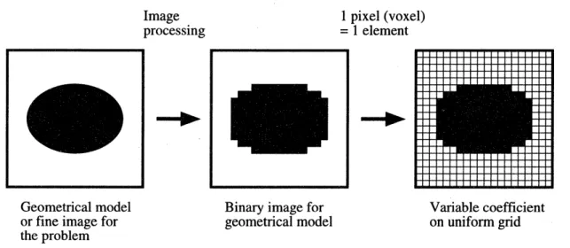
In the image-based$\mathrm{a}\mathrm{p}\mathrm{p}\mathrm{r}\mathrm{o}\mathrm{a}\mathrm{c}\mathrm{h}[1]$, the bit-mapinformation ofthe digital imageofstructures

is usedasageometrical model, and each volume element (voxel) in the image is recognized

as a finite element in the uniform rectangular grid (see fig. 1).

Image 1 pixel(voxel)

processing $=1$ element

Geometrical model Binary imagefor Variable coefficient

orfineimagefor geometrical model onuniformgrid

theproblem

Fig. 1 Image-based Finite Element method

Inthe image-based approach, very fine gridisrequiredto representcomplex geometry. In our target problem of concrete materials, the number ofdegrees of freedom becomes

$10^{6}$ to $10^{8}$. In the nonlinear simulation based on the image-based approach, such a huge

linear system need to be solved many times. Therefore developmentof the fast solver for

such a huge linear system is the key to apply the image-based finite element method to the nonlinear simulation.

However, the image-based approach offers the feature of uniform rectangular grid. Owing to this property, sophisticated but restrictive procedures thatare difficult to apply to the conventional finite element method using unstructured meshes can be applied to solve the linear system arising in the image-based approach.

In this work, two types of iterative solvers led by the feature of uniform rectangular grid are considered as follows:

1. Conjugate gradient method with effective preconditioner using signal processing technique

2. Multigrid method

2.2

Preconditioned

Conjugate

Gradient

Method

The best iterative solver for the elasticity shouldbe the conjugate gradient $(\mathrm{C}\mathrm{G})$ method. As is widely known, an effective preconditioner can be designed by using the good ap-proximation of the inverse matrix. Our problem is basically elasticity, which is of second

order elliptic problem. The mathematical propertyofthe problem is similar to the

Pois-son equation. Thus the Poisson solver is a candidate of the effective preconditioner. Well-known fast Poisson solvers arebased onthe spectralmethod. In the image-based finite element method, all the unknown variable is on the uniform grid, and it can be recognized as the variable on the uniform sampling points. In such a situation, the fast Poisson solver using signal processing techniques such as fast Fourier transform (FFT)

or wavelet transform to precondition the matrix can be employed. Signal processing

techniques are widely used and various efficient algorithms have been developed in the field of the computer science. Therefore a fast iterative solver for the image-based FEM

can be constructed by using such techniques.

In this work, the FFT is employed to construct the fast Poisson solver and its is applied to the components of theresidualvector corresponding to each physical direction. In other words, the fast Poisson solver, which consists of one Fourier transform, scaling

in the frequency domain and an inverse transform, are performed three times to obtain

an improved direction vector from a residual vector in the three dimensional problem. In this paper, this procedure is called FFT preconditioned CG (FFT-PCG) method.

2.3

Cascadic

Conjugate Gradient

Method

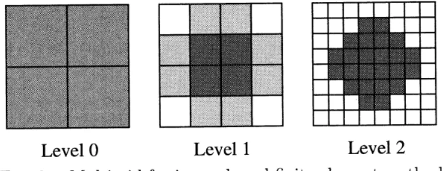
For the uniformrectangular grid used in the image-based approach, a sequence of nested finite element spaces for the multigridmethod can be constructedeasily as shown in Fig. 2. Thus the multigrid method is worth considering to develop a fast iterative solver.

There aredifferenttypesof iterative procedures based onthe multigridmethod, which

are categorized by their iterative process between fine grid and

coarse

grid. Typical

ones

are known as $\mathrm{V}$-cycle or $\mathrm{W}$-cycle. Recently the cascadic multigrid method was

developed by $\mathrm{D}\mathrm{e}\mathrm{u}\mathrm{f}\mathrm{l}\mathrm{h}\mathrm{a}\mathrm{r}\mathrm{d}[4]$ . The iterative process in the cascadic multigrid method are

performed from

coarse

grid to fine one in one way. Thus it is sometimes called one-way multigrid method. In this work, the cascadic conjugate gradient (CCG) $\mathrm{m}\mathrm{e}\mathrm{t}\mathrm{h}\mathrm{o}\mathrm{d}[4]$,

Level$0$ Level

1

Level

2

in which the conjugate gradient method is used as the basic iteration, is applied to the image-based finite element method. This method is based on the fact that both the iteration of multigrid sequence for the Galerkin finite element approximation and that of the conjugate gradient method are known to minimize the energy norm arising iteration

errors.

Actually the

CCG

method consists of the two nested iterations. The outer iteration is for the multigrid, while the inner is for the conjugate gradient method. The iteration control mechanism is based on the approximated energy

error

norm and it makes the CCG efficient. Although this procedure is very simple, it has been shown to be efficient owing to such mathematical background.

3

Numerical

experiments

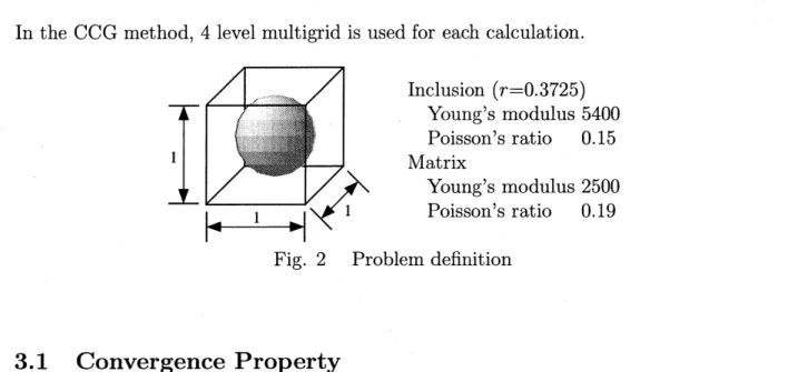
In order to evaluate numerical properties of the present methods, the problem derived from the homogenization method for composite materials is solved. A simple composite

material with a spherical inclusion in the representative volume element (RVE) as shown

in Fig. 2 is considered and the characteristicfunctioncorresponding to the uniform axial strain iscalculated. In this problem, the periodic boundary condition is subjected to each surface on the RVE and a body force is imposed. In this work, three cases with different meshes $(32^{3},64^{3},963)$ are calculated. The termination criteria for the FFT-PCGmethod

is specified by the $L^{2}$ norms of residual $\mathrm{r}$ and external force vector $\mathrm{f}$ as

$||\mathrm{r}||_{L^{2}}\leq 10^{-5}||\mathrm{f}||_{L^{2}}$

.

In the CCG method, 4 level multigrid is used for each calculation. Inclusion $(r=0.3725)$ Young’s modulus 5400 Poisson’s ratio $0.15$ Matrix Young’s modulus 2500 Poisson’s ratio 0.19

Fig. 2 Problem definition

3.1

Convergence

Property

Table 1 shows the numbers of iterations needed for the convergence in the FFT-PCG

method. These numbers indicate that the number of iterations is independent to the problem size in the FFT-PCG method.

Table 2 shows the numbers of iterations for each grid level in the CCGmethod. Every inner CG process requires small number of iterations which are almost independent to

Ta$\mathrm{h}1‘ 1\rceil$ $\mathrm{N}1\rceil \mathrm{m}\mathrm{h}\rho r$ nf$\mathrm{i}\mathrm{f}.\rho\gamma \mathrm{a}\dotplus \mathrm{i}\cap \mathfrak{n}.\mathrm{Q}$ in Pa$\Gamma_{\mathrm{v}}\mathfrak{m}\rho+.\mathrm{h}\mathrm{o}\mathrm{d}$

Table 2 Number of iterations in CCG method (4 level)

the problem size. The numbers of iterations corresponding to the final level are smaller than those indicated in FFT-PCG method.

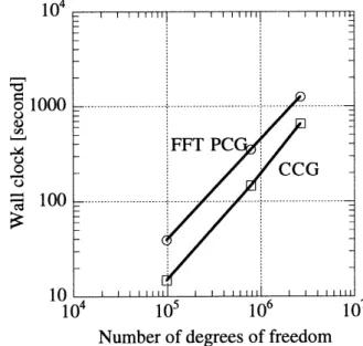
Overallcomputational costsareevaluated for the FFT-PCG andCCG methods. From Fig. 3 that shows the elapsed time, the CCG method is 50% faster that FFT-PCG

method. This is due to the fact that 3 dimensional fast Fourier transform is performed in the preconditioning process of the FFT-PCG method and its computational cost is not small.

Numberofdegreesot$\iota \mathrm{r}\mathrm{e}\mathrm{e}\mathrm{d}\mathrm{o}\mathrm{m}$

3.2

Parallel Performance

on

PC Cluster

In this work, parallel performance of the present procedures is also compared by using

Beowulftype PC $\mathrm{c}\mathrm{l}\mathrm{u}\mathrm{s}\mathrm{t}\mathrm{e}\mathrm{r}[5]$, whichis aparallel computer consistingofpersonal computers

connected byEthernet. The specification of

our

PC clusteris shown inTable 3. To carry

out parallelprocessing, the problem domain isdivided into slabsof which number is equal to that of processors.

Table 3 $\mathrm{s}\mathrm{D}\mathrm{e}\mathrm{c}\mathrm{i}\mathrm{f}\mathrm{i}\mathrm{C}\mathrm{a}\mathrm{t}\mathrm{i}_{\mathrm{o}\mathrm{n}}$ of PC

cluster

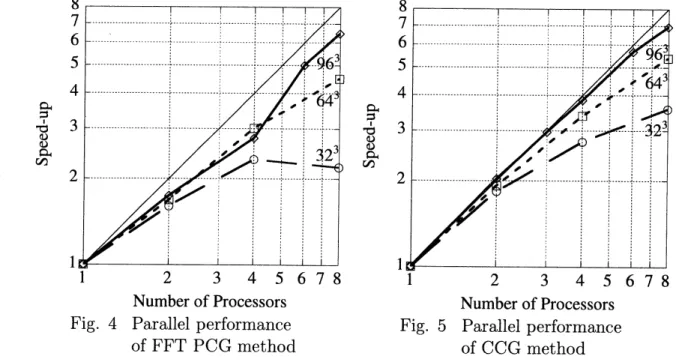
Figure4 and 5 show the scalability of thepresent procedureon the parallelprocessing. The CCG method exhibits good _{scalability, since most of the communications between}

processors in the CCG method is neighboring. On the other hand, the scalability of

FFT-PCG method is worth than that of the CCG method especially in the small case.

In the FFT-PCG method, _{FFT stage requires all to all communication in which every} node needs to communicate to all the rest of it. Thus the narrow band width of the

network in the PC cluster decrease the scalability of FFT-PCG method.

$3\approx$ $3^{4}\mathfrak{Q}$ $\mathrm{r}^{1}$ $\mathrm{q})0$ $\approx\Phi \mathrm{d}\mathrm{J}$ $\infty\alpha$ $\infty\approx$ Numoer

or

$\mathrm{P}\mathrm{r}\mathrm{o}\mathrm{C}\mathrm{e}\mathrm{s}\mathrm{S}\mathrm{o}\mathrm{r}\mathrm{s}$ Numoerot Processors

Fig. 4 Parallel performance Fig. 5 Parallel performance

4

Concluding

Remarks

In this work, two different types of iterative solvers for the image-based finite element method are evaluated. Both the FFT-PCG and CCG methods exhibit almost optimal complexity in the numerical experiment. In the view of both the serial and parallel processing, the CCG method is superior to the FFT-PCG method.

References

[1] S.J. Holister and N. Kikuchi, ”homogenization theory and digital imaging: a basis for studyingthe mechanics and design principles ofonetissue”, Biotech. Bioeng.43(1994),

586-596.

[2] G.Nagai, T.Yamada and A.Wada, ”Stress analysis of concrete material based on geometrically accurate finite element method,” Proc.

_Conf.

Comp. Engng. Sci., 2 (1997), 1103-1106 (in Japanese).

[3] G.Nagai, T.Yamada and A.Wada, ”_{Finiteelement analysis of concrete material based}

on the image data,” Proc. FRAMCOS 3, 2 (1998), 1077-1086.

[4] P. Deuflhard, ”_{Cascadic conjugate gradient methods for} elliptic partial differential

Equation. Algorithm and numerical results”, In D. Keyes and J. Xu, editors, Proc. 7th Int.

_Conf.

Domain Decomposition Methods 1993,(1994) 29-42.